9 Classification of Genomic and Proteomic Data Using Support Vector ...

9 Classification of Genomic and Proteomic Data Using Support Vector Machines Peter Johansson and Markus Ringn´er Computational Biology and Biological Physics Group, Dept. of Theoretical Physics, Lund University, Sweden [email protected], [email protected]

9.1 Introduction Supervised learning methods are used when one wants to construct a classifier. To use such a method, one has to know the correct classification of at least some samples, which are used to train the classifier. Once a classifier has been trained it can be used to predict the class of unknown samples. Supervised learning methods have been used numerous times in genomic applications and we will only provide some examples here. Different subtypes of cancers such as leukemia (Golub et al., 1999) and small round blue cell tumors (Khan et al., 2001) have been predicted based on their gene expression profiles obtained with microarrays. Microarray data has also been used in the construction of classifiers for the prediction of outcome of patients, such as whether a breast tumor is likely to give rise to a distant metastasis (van ’t Veer et al., 2002) or whether a medulloblastoma patient is likely to have a favorable clinical outcome (Pomeroy et al., 2002). Proteomic patterns in serum have been used to identify ovarian cancer (Petricoin et al., 2002a) and prostate cancer (Adam et al., 2002; Petricoin et al., 2002b). In this chapter, we will give an example of how supervised learning methods can be applied to high-dimensional genomic and proteomic data. As a case study, we will use support vector machines (SVMs) as classifiers to identify prostate cancer based on mass spectral serum profiles.

9.2 Basic Concepts In supervised learning the aim is often to construct a rule to classify samples in pre-defined classes. The rule is constructed by learning from learning samples. The correct class assignments are known for the learning data and used in the construction of the rule. The number of samples needed to construct a classification rule is data set and classification method dependent. In our

2

Peter Johansson and Markus Ringn´er

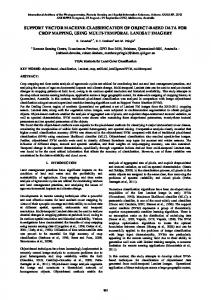
experience at least ten samples in each class are needed for classification of genomic and proteomic data. Once the rule is constructed it can be applied to classify unknown samples. Each sample typically is a vector of real values and each value often corresponds to a measurement of one feature of the sample. Classification rules can be either explicit or implicit. An example of a classification method with an implicit rule is the nearest neighbor classifier: A test sample is classified to belong to the same class as the learning sample to which it is most similar. Decision trees are a classification method that use explicit rules, for example, if the value of a specific feature of the sample is positive, the sample is predicted to belong to one class, if not, it is predicted to belong to another class. In the case of classifying tumor samples based on genomic or proteomic data, each sample could, for example, be a vector of gene expression levels from a microarray experiment, volumes from spots on a 2dimensional gel, or intensities for different mass-over-charge (m/z) values from a mass spectrum. Classes could, for example, be cancer patients and healthy individuals, respectively. In these cases, data sets have very many features and it is often beneficial to separate construction of the classifier in two parts: feature selection and classifier rule construction. Moreover, once a classifier is constructed its predictive performance needs to be evaluated. In this section, we will discuss a supervised learning method: SVM, how feature selection can be combined with SVMs, and a methodology for obtaining estimates of the predictive performance of the classifier. 9.2.1 Support Vector Machines Suppose we have a set of samples where each sample belongs to one of two pre-defined classes, and we have measured two values for each sample, for example, the expression levels of two proteins (Figure 9.1). Two classes of two-dimensional samples are considered linearly separable if a line can be constructed such that all samples of one class lie on one side of the line and all samples of the other class lie on the other side. This line serves as a decision boundary between the two classes. For higher-dimensional data, a linear decision boundary is a hyperplane that separates the classes. If classes are separable by a hyperplane, there are most likely many possible hyperplanes that separate the classes (Figure 9.1a). SVMs are based on this concept of decision boundaries. SVMs are designed to find the hyperplane with the largest distance to the closest points from the two classes, the maximal margin hyperplane (Figure 9.1c). Once this hyperplane has been found for a set of learning samples, the class of additional test samples can be predicted based on which side of the hyperplane they appear. For many classification problems the classes cannot be separated by a hyperplane; they are not linearly separable and a non-linear decision surface may be useful. Classifiers that use a non-linear decision surface are called non-linear classifiers. SVMs address such classification problems by mapping the data from the original input space into a feature space in which a linear

9 Classification Using Support Vector Machines

Feature 2

(c)

Feature 1

Feature 2

(b)

Feature 2

(a)

3

Feature 1

Feature 1

Fig. 9.1. Finding the separating hyperplane with the maximal margin for the linearly separable case. A data set consisting of 10 samples with 2 features each is classified. Each sample belongs to one of two different classes (denoted by + and •, respectively). A linear decision boundary is a hyperplane separating the two classes. In the case of two features such a hyperplane is a line. Many hyperplanes exist that perfectly separate the samples from the two classes (a). Suppose we draw circles with the same diameter around each sample and that the separating hyperplanes are not allowed to intersect the circles. It is then obvious that with an increasing diameter of the circles, the number of allowed hyperplanes decreases (b). The diameter is increased until only one hyperplane exist (c). This hyperplane is completely defined by the points encircled by solid circles and these points are called support vectors. Intuitively this final hyperplane seems more appropriate as a decision boundary because it maximizes the margin between the two classes. SVMs are designed to find this maximal margin hyperplane.

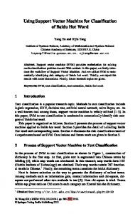
separator can be found. This mapping does not need to be explicitly specified. Instead a user of SVMs needs to select a so-called kernel function, which can be viewed as a distance between samples in feature space (Figure 9.2). The linear decision surface in feature space may correspond to a non-linear separator in the original input space. To avoid over-fitting to data, avoid sensitivity to outlier samples, or handle problems that are not linearly separable in feature space, SVMs with soft-margins can be used. For such SVMs the strict constraint to have perfect separation between the classes is softened. A parameter denoted C is introduced to tolerate errors. The larger C is, the harder errors are penalized. The limit of C being infinity corresponds to the maximal margin case for which no errors are tolerated. For microarray and proteomic data, for which the number of features is much larger than the number of samples, it is typically possible to find a linear classifier that perfectly separates the samples. It is our experience for highdimensional data that SVMs with a linear kernel and the C parameter set to infinity results in classifiers with better predictive performance than SVMs for which one tries to optimize kernel selection and C parameter value. An SVM with this choice of parameters is called a linear maximal margin classifier.

4

Peter Johansson and Markus Ringn´er

1

1

x1 x 2

(b)

x2

(a)

0

-1

0

-1 -1

0

x1

1

-2

0

2

x1 + x2

Fig. 9.2. Mapping the XOR problem into a feature space in which it is linearly separable. A data set consisting of 20 samples with two features each and belonging to two different classes (denoted by + and •, respectively) is shown. (a) The two classes are not linearly separable in the original input space (x1 , x2 ). (b) The input space can be mapped to the feature space (x1 + x2 , x1 x2 ), where the two classes are linearly separable. The kernel for this mapping is K(a, b) = (a1 + a2 )(b1 + b2 ) + a1 a2 b1 b2 .

9.2.2 Feature Selection The amount of information contained in a mass spectrum, or the number of genes measured on a microarray, results in very many features for each sample. When the number of features is much larger than the number of samples, it represents a challenge for many supervised learning methods. This problem is often referred to as the “curse of dimensionality”. To address this problem, feature selection techniques are used to reduce the dimensionality of the data to improve subsequent classification. Feature selection methods can be divided into two broad categories: Wrapper methods and filter methods. Wrapper methods evaluate feature relevance within the context of the classification rule. For example, by first constructing a classification rule using all features, and then analyzing the classification rule to identify the features most important for the rule, followed by constructing a new classification rule using only these important features. A wrapper method used with SVMs is recursive feature elimination (Guyon et al., 2002). Filter methods select features based on a separate criterion unrelated to the classification rule. For example, the standard two-sample t-test could be used as a filter criterion for two class classification problems to identify and rank features that discriminate between the two classes. Another commonly used filter selection criteria used to rank features is the signal-to-noise ratio (S2N ratio) (Golub et al., 1999). Here each feature is ranked based on S2N = |µ+ −µ− |/(σ+ −σ− ), where µ± and σ± are the average and standard deviation, respectively, of the values for the feature in the two classes + and − (see Equation(7.1), Chapter 7). A classification rule is then constructed using only the features that have the largest S2N.

9 Classification Using Support Vector Machines

5

Filter methods have been shown to provide classification performances that are comparable to or outperform other selection methods for both microarray and mass spectronomy data (Wessels et al., 2005; Levner, 2005). In our experience t-test and S2N perform similarly and the choice of the filter criterion is not crucial. 9.2.3 Evaluating Predictive Performance To evaluate the predictive performance of a classifier, one needs a test set that is independent of all aspects of classifier construction. If the number of samples investigated is relatively small, one often resorts to cross-validation. In n-fold cross-validation, the samples are randomly split into n groups of which one is set aside as a test set and the remaining groups are a learning set used to calibrate a classifier. The procedure is then repeated with each of the n groups used as a test set. Finally, the samples can again be randomly split into n groups and the whole procedure repeated many times. These test sets would provide a reliable estimate of the true predictive performance, if there were no choices in classifier construction. An example of such a case is if one, prior to any data analysis, decides to use an SVM with linear kernel, C set to infinity, and all features (no feature selection). However, suppose one only wants to use the features that provide the best prediction results, then the test set is no longer independent because it has been used to optimize the number of features to use in the classification rule. To circumvent this use of the test set, the learning samples can be used to optimize the prediction performance of the classifier in an internal procedure of cross-validation. This internal nfold cross-validation is identical to the cross-validation used for generating test sets, except that one group of samples is used to optimize the performance of the classifier (validation set) and the remaining samples are used to train the classifier (training set). Hence, these cross-validation samples will provide an overly optimistic estimate of the predictive performance (Ambroise and McLachlan, 2002). Once all the choices required to construct a classifier has been made in the internal cross-validation, the performance can be evaluated on the samples set aside in the external cross-validation loop. A schematic picture of this procedure is given in Figure 9.3. The number of folds used in the external and internal cross-validations can be different. To assess if a predictive performance achieved by SVMs is significant random permutation tests can be used. In these tests the predictive performance is compared to results for SVMs applied to the same data but with the class labels randomly permuted (Pavey et al., 2004).

6

Peter Johansson and Markus Ringn´er

(a)

External cross-validation

1

2

3

4

5

6

7 8

Learning

(b)

9

Test

Internal cross-validation

1

2

3

4

Training

5

6

Validation

Fig. 9.3. One fold in an (a) external and (b) internal 3-fold cross-validation procedure. In total, the data set comprises nine samples, each represented by a number. The external cross-validation is used to estimate the predictive performance of the classifier and the internal cross-validation is used to optimize the choices made when constructing the classifier. The samples belong to two classes, gray and white. For both the internal and external cross-validation, the folds are stratified to approximate the same class distributions in each fold as in the complete data set.

9.3 Advantages and Disadvantages 9.3.1 Advantages ˆ

SVMs perform non-linear classification by mapping data into a space where linear methods can be applied. In this way, non-linear classification problems can be solved relatively fast computationally.

9.3.2 Disadvantages ˆ

SVMs may be too sophisticated for many genomic and proteomic classification problems (Somorjai et al., 2003). Occam’s razor principle tells us to prefer the simplest method and often linear SVMs give the best classification performance, in which case alternative linear classification methods may be more easily applied.

9.4 Caveats and Pitfalls The two most important aspects of classification of genomic and proteomic data are not directly related to the choice of classification method. First, high-quality data needs to be obtained, in which biologically relevant features are not confounded by experimental flaws. Second, a proper methodology

9 Classification Using Support Vector Machines

7

to evaluate the classification performance needs to be implemented to avoid overly optimistic estimates of predictive performances, or more importantly, to avoid finding a classification signal when there is none (Simon et al., 2003). When estimating the true predictive performance using a test data set, it is crucial to use a procedure, in which the test data is not used to select features, to construct the classification rule, or even to select the number of features to use in the classifier. In the case study, we will see how the violation of these requirements influences classification results.

9.5 Alternatives Nearest centroid classifiers provide an alternative to SVMs that are simple to implement and have been used successfully for many genomic applications (van ’t Veer et al., 2002; Tibshirani et al., 2002; Wessels et al., 2005). For this type of classifiers there exists available software tailored for genomic and proteomic data. Therefore, we describe how a simple version is implemented. First, the arithmetic mean for each feature is calculated using only samples within each class. In this way a prototype pattern for each class called a centroid is obtained. Second, one defines a distance measure between samples and centroids, and the classes of additional test samples are predicted by calculating to which centroid they are nearest. There are many supervised learning methods that can be applied to genomic and proteomic data, including linear discriminant analysis, classification trees, and nearest neighbor classifiers (Dudoit et al., 2002), as well as artificial neural networks (Khan et al., 2001).

9.6 Case Study: Classification of Mass Spectral Serum Profiles Using Support Vector Machines As a case study, we applied SVMs to a public data set of mass spectral serum profiles from prostate cancer patients and healthy individuals (Petricoin et al., 2002b) to see how well the disease status of these individuals could be predicted. 9.6.1 Data Set The data set consists of 322 samples: 63 samples from individuals with no evidence of disease, 190 samples from individuals with benign prostate hyperplasia, 26 samples from individuals with prostate cancer and PSA levels 4 through 10, and 43 samples from individuals with prostate cancer and PSA levels above 10. For our case study, we followed previous analysis (Levner, 2005) and combined the two first groups into a healthy class containing 253 samples, and the latter two groups into a disease class containing 69 samples.

8

Peter Johansson and Markus Ringn´er

For each individual, a mass spectral profile of a serum sample has been generated using surface-enhanced laser desorption ionization time-of-flight (SELDI-TOF) mass spectrometry (Hutchens and Yip, 1993; Issaq et al., 2002). In this method, a serum sample taken from a patient is applied to the surface of a protein-binding chip. The chip binds a subset of the proteins in the serum. A laser is used to irradiate the chip resulting in the proteins being released as charged ions. The time-of-flights of the charged ions are measured providing an m/z value for each ion. Each sample will in this way give rise to a spectrum of intensity as a function of m/z; a proteomic signature of the serum sample. The data set used in our case study consists of spectra with intensities for 15,154 m/z values. Hence, the number of features (15,154) is much larger than the number of samples (322). 9.6.2 Analysis Strategies We used linear SVMs with C set to infinity (linear maximal margin classifiers). The predictive performance was evaluated using 5 times repeated 3-fold external cross-validation, which resulted in a total of 15 test sets, each with one-third of 322 samples. The cross-validation was stratified to approximate the same class distributions in each fold as in the complete data set. We used S2N to rank features and classifiers using different numbers of top-ranked features (nf ) were evaluated. A set of classifiers was constructed, in which each classifier was trained using 1.5 × nf more top-ranked features than the previous classifier; the first classifier used the top-ranked feature (nf = 1) and the final classifier used all features. The performance of classifiers was evaluated using the balanced accuracy (BACC). Given two classes, 1 and 2 with N1 and N2 samples, respectively, we denote samples known to belong to class 1 as true positives (TP) if they are predicted to belong to class 1, and false negatives (FN) if they are predicted to belong to class 2. Correspondingly, samples known to belong to class 2 are true negatives (TN) if they are predicted to belong to class 2 and false negative (FN) otherwise. BACC is the average of the sensitivity and the specificity, in other words, it is the average of the fractions of correctly classified samples for each of the two classes: µ ¶ µ ¶ TP TN 1 TP TN 1 + = + (9.1) BACC = 2 TP + FN TN + FP 2 N1 N2 An advantage of BACC is that a simple majority classifier that predicts all samples into the most abundant class will obtain a BACC of 50% even though it is expected to obtain overall classification accuracies, (TP+TN)/(N1 +N 2), higher than 50%. We used four different strategies to construct SVMs : Two strategies in which the test sets were independent of all aspects of SVM construction, and two strategies exemplifying how overly optimistic estimates of the predictive power can be obtained (Figure 9.4).

9 Classification Using Support Vector Machines

(a)

(c)

External cross-validation 2

3

4

5

6

7

1

9

3

2

4

5

6

Test

Learning

Independent test

Select nf features

Learning

Train SVM

8

External cross-validation

Optimize nf

1

9

7

8

9

Test

Train SVM Validate SVM Dependent test

(b)

(d)

External cross-validation

1 2

3

4

5

6

7

Learning

8

2

3

4

Training

5

6

Validation

Select nf features Optimize nf

3

4

5

6

7 8

9

Total

Test

Train SVM Find optimal number using nopt features of features: nopt Independent Internal cross-validation test 1

2

9

Select nf features External cross-validation Optimize nf

1

1

2

3

4

5

6

Learning

7

8

9

Test

Train SVM Validate SVM

Train SVM Dependent test Validate SVM

Fig. 9.4. The four strategies used to construct SVMs. In strategies A and B the test samples are not used for training SVMs, for feature selection, or for optimizing the number of features to use. Hence, a good estimate of the true predictive performance may be obtained using strategies A or B. In strategy C the test samples are used to select the number of features to use. In strategy D the test samples are used both to select features and to optimize the number of features to use. Hence, an overly optimistic estimate of the true predictive performance is obtained using strategies C or D.

10

Peter Johansson and Markus Ringn´er

9.6.2.1 Strategy A: SVM without Feature Selection An SVM is trained using all the learning samples and all features (Figure 9.4a). 9.6.2.2 Strategy B: SVM with Feature Selection Internal 3-fold cross-validation is used to optimize the number of features, nopt , to use for the learning set. In the internal cross-validation, the learning samples are split into a group of training samples and a group of validation samples. SVMs are trained using the training samples and nf top features ranked based only on these samples. The internal cross-validation is performed one round (a total of three validation sets) such that each learning sample is validated once. The performance in terms of BACC for the validation data is used to select an optimal nf . Finally, an SVM is trained using all learning samples and the nopt top-ranked features based on these learning samples. This final SVM is used to predict the classes of the test data samples (Figure 9.4b). 9.6.2.3 Strategy C: SVM Optimized Using Test Samples Performance SVMs are trained using the learning samples and nf top features ranked based only on these samples. The performance in terms of BACC for the test data is used to evaluate the number of features to use. The predictions for the test data samples by the SVM with the optimal performance is used. Here the test performance is an overly optimistic estimate of the true predictive performance since the test data is used to find nopt (Figure 9.4c). 9.6.2.4 Strategy D: SVM with Feature Selection Using Test Samples SVMs are trained using the learning samples and nf top features ranked based on all samples. The performance in terms of BACC for the test data is used to evaluate the number of features to use. The predictions for the test data samples by the SVM with the optimal performance is used. Here the test performance is an overly optimistic estimate of the true predictive performance since the test data is used both to find nopt and to rank features (Figure 9.4d). 9.6.3 Results The results in terms of BACC for the four different strategies is summarized in Table 9.1.

9 Classification Using Support Vector Machines

11

Table 9.1. Predictive performance of SVMs BACC(%)b Mean Std A: SVM without feature selection 88.7 3.6 B: SVM with feature selection 91.1 3.3 C: SVM optimized using test sample performance 94.6 2.6 D: SVM with feature selection using test samples 94.9 1.8 Strategy

a

a b

See Analysis Strategies in section 9.6. Balanced accuracy: average of sensitivity and specificity.

9.7 Lessons Learned We have shown an example of how SVMs are capable of predicting with high accuracy whether mass spectral serum profiles belong to a healthy or a prostate cancer class. High balanced accuracy (88.7%) was obtained without any feature selection, yet a simple filter selection method improved the predictive performance and a BACC of 91.1% was obtained. This BACC is competitive with the best performance obtained for this data set in a study of different feature selection methods (Levner, 2005). In the context of crossvalidation it is difficult to evaluate if a method is significantly better than another method because different test sets have samples in common (Berrar et al., 2006). There are many pitfalls when evaluating the predictive performance of classifiers. By using the test data simply to select the number of features to use by the classification rule, the BACC increased to 94.6%. This performance is an overly optimistic estimate of the true predictive performance not likely to be achieved for independent test data. Similarly, overly optimistic results were obtained when the test data was used to rank features prior to feature selection. It is important to realize that overly optimistic evaluations may lead to incorrect conclusions for classes which cannot be classified (Ambroise and McLachlan, 2002; Simon et al., 2003).

9.8 List of Tools and Resources There are several publicly available implementations of SVMs and a comprehensive list is available at http://www.kernel-machines.org/software.html. For example, there is an implementation in C called SVMLight (http://svmlight.joachims.org/) and an implementation called LIBSVM with interfaces to it for many programming languages (http://www.csie.ntu.edu.tw/~cjlin/libsvm). In the case of microarray data analysis, SVMs are available as a part of the TM4 microarray software suit (http://www.tm4.org/). Publicly available implementations of nearest centroid classifiers include ClaNC (Dabney, 2006);

12

Peter Johansson and Markus Ringn´er

http://students.washington.edu/adabney/clanc/) and PAM (Tibshirani et al., 2002); http://www-stat.stanford.edu/~tibs/PAM/), both implemented for the R package (http://www.r-project.org).

9.9 Conclusions SVMs can be used to classify high-dimensional data such as microarray or proteomic data. Often the simplest SVMs called maximal margin linear SVMs are able to obtain high accuracy predictions. For many applications it is important to evaluate classifiers based on their predictive performance on test data. In this evaluation, it is important to implement test procedures that do not lead to overly optimistic results. We have used mass spectral serum profiles of prostate cancer patients and healthy individuals as a case study to exemplify how the predictive performance of a classifier can be estimated. We conclude that SVMs predict the samples in our case study with high balanced accuracy.

9.10 Appendix: Outline of Mathematical Details We will consider the simplest version of a support vector machine, the socalled linear maximal margin classifier for classification of data points in two classes. This classifier only works for data points which are linearly separable. Two classes of two-dimensional samples are considered linearly separable if a line can be constructed such that all cases of one class lie on one side of the line and all cases of the other class lie on the other side. For a more detailed description of SVMs, there are many books available for the interested reader (Vapnik, 1995; Burgess, 1998; Cristianini and Shawe-Taylor, 2001). Consider a linearly separable data set {(xi , yi )}, where xi are the input values for the ith data point and yi is the corresponding class {−1, 1}. The assumption, that the data set is linearly separable, means that there exists a hyperplane that separates the data points of the two classes without intersecting the classes. This hyperplane serves as a decision surface, and we can write: w0 xi + b ≥ 0 i : yi = +1 w0 xi + b ≤ 0 i : yi = −1 , where the hyperplane is defined by w and b, and w0 x+b is the output function. The distance from the hyperplane to the closest point is called the margin (denoted by γ). The underlying idea of the maximal margin classifier is that, in order to have a good classifier, we want the margin to be maximized. We notice there is a free choice of scaling: Rescaling (w, b) to (λw, λb) does not change the classification given by the output function. The scale is to set such that

9 Classification Using Support Vector Machines

13

w0 x+ + b = +1 w0 x− + b = −1 ,

(9.2)

where x+ (x− ) is the closest data point on the positive (negative) side of the hyperplane. Now it is straightforward to compute the margin µ ¶ 1 w0 x+ + b w0 x− + b 1 γ= − = . 2 kwk kwk kwk Hence, when the scale is set such that Equation (9.2) is fulfilled then maximizing the margin is equivalent to minimizing the norm of the weight vector, kwk. This can be formulated as a quadratic (w0 w) problem with inequality constraints (yi (w0 xi + b) ≥ 1): min:

1 0 ww 2

subject to: yi (w0 xi + b) ≥ 1 for all yi .

The Lagrangian for this quadratic problem is L(w, b, α) =

M X 1 0 ww− αi [yi (w0 xi + b) − 1] , 2 i=1

(9.3)

where αi ≥ 0 are the Lagrange multipliers and M is the number of data points. Differentiating with respect to w and b and setting the partial derivatives to zero give M

X ∂L =0⇒w= αi yi xi ∂w i=1

(9.4)

M X ∂L =0⇒ yi αi = 0 , ∂b i=1

(9.5)

and putting this into Equation (9.3) gives the Wolfe dual     M M M M X X X 1X Q(α) = αi yi x0i αj yj xj − αi yi  αj yj x0j xi + b − 1 2 i=1 j=1 i=1 j=1 M X 1 αi , = − α0 Hα + 2 i=1

(9.6)

where the elements of the matrix H are given by Hij = yi yj x0i xj .The original problem is transformed into a dual problem. Finding the dual vector, α, that maximizes Q and fulfills the constraint in Equation (9.5) is equivalent to solving the original problem (Kuhn and Tucker, 1951). The output of the classifier for a data point x can be expressed in terms of the dual vector

14

Peter Johansson and Markus Ringn´er

o(x) = w0 x + b =

M X

αi yi x0i x + b ,

(9.7)

i=1

and we note that the weight vector is never needed explicitly. The variable b is set such that the conditions in Equation (9.2) are fulfilled. The binary classification of a data point x is sign(o(x)). The hyperplane that separates the data points is completely defined by a subset of the data points and these data points are called support vectors (Figure 9.1). Each αi corresponds to a learning data point xi and αi is zero for all data points except the support vectors. Hence the sum in Equation (9.7) only gets contributions from the support vectors. In summary, there are three steps to build and use a maximal margin classifier. First, the class labels of the learning data points should be set to +1 or −1. Second, the quadratic function in Equation (9.6) is minimized subject to the constraint in Equation (9.5) and all αi ≥ 0. Because the matrix H in Equation (9.6) is positive definite there are no local minima and there is a unique solution to the minimization problem. Finally, this solution is used to classify data points in a validation/test set using Equation (9.7). We conclude by briefly outlining how to extend this linear classifier to nonlinear SVMs. The basic idea underlying non-linear SVMs is to map data points into a feature space in which an optimal hyperplane can be found as outlined for the maximal margin classifier. This hyperplane may then correspond to a non-linear separator in the original space of data points. A key observation is that in our construction of the maximal margin classifier we only use the scalar product between data points, x0i xj . If we have a non-linear mapping, x 7→ ϕ(x), of data points into feature space, the scalar product between two vectors in feature space, called a kernel function, is X ϕl (xi )ϕl (xj ) . K(xi , xj ) = ϕ(xi )0 ϕ(xj ) = l

In SVMs, the scalar product between data points used to calculate both H and o(x) is replaced by the kernel K. Hence, to build and use an SVM, the mapping into feature space itself can be ignored and only a kernel function needs to be defined.

9 Classification Using Support Vector Machines

15

References Adam, Bao-Ling, Qu, Yinsheng, Davis, John W, Ward, Michael D, Clements, Mary Ann, Cazares, Lisa H, Semmes, O John, Schellhammer, Paul F, Yasui, Yutaka, Feng, Ziding, and Wright, George L Jr (2002). Serum protein fingerprinting coupled with a pattern-matching algorithm distinguishes prostate cancer from benign prostate hyperplasia and healthy men. Cancer Res, 62(13):3609–3614. Ambroise, Christophe and McLachlan, Geoffrey J (2002). Selection bias in gene extraction on the basis of microarray gene-expression data. Proc Natl Acad Sci U S A, 99(10):6562–6566. Berrar, Daniel, Bradbury, Ian, and Dubitzky, Werner (2006). Avoiding model selection bias in small-sample genomic datasets. Bioinformatics, 22(10):1245–1250. Burgess, C J C (1998). A tutorial on support vector machines for pattern recognition. Data Mining and Knowledge Discovery, 2(2):121–167. Cristianini, N. and Shawe-Taylor, J. (2001). An introduction to Support Vector Machines and other kernel-based learning methods. Cambridge University Press. Dabney, Alan R (2006). ClaNC: point-and-click software for classifying microarrays to nearest centroids. Bioinformatics, 22(1):122–123. Dudoit, S, Fridlyand, J, and Speed, T P (2002). Comparison of discrimination methods for the classification of tumors using gene expression data. JASA, 97:77–87. Golub, T R, Slonim, D K, Tamayo, P, Huard, C, Gaasenbeek, M, Mesirov, J P, Coller, H, Loh, M L, Downing, J R, Caligiuri, M A, Bloomfield, C D, and Lander, E S (1999). Molecular classification of cancer: class discovery and class prediction by gene expression monitoring. Science, 286(5439):531–537. Guyon, Isabelle, Weston, Jason, Barnhill, Stephen, and Vapnik, Vladimir (2002). Gene Selection for Cancer Classification using Support Vector Machines. Machine Learning, 46:389–422. Hutchens, T W and Yip, T T (1993). New desorption strategies for the mass spectrometric analysis of macromolecules. Rapid Commun Mass Spectrom, 7:576–580. Issaq, Haleem J, Veenstra, Timothy D, Conrads, Thomas P, and Felschow, Donna (2002). The SELDI-TOF MS approach to proteomics: protein profiling and biomarker identification. Biochem Biophys Res Commun, 292(3):587–592. Khan, J, Wei, J S, Ringner, M, Saal, L H, Ladanyi, M, Westermann, F, Berthold, F, Schwab, M, Antonescu, C R, Peterson, C, and Meltzer, P S (2001). Classification and diagnostic prediction of cancers using gene expression profiling and artificial neural networks. Nat Med, 7(6):673–679. Kuhn, H. and Tucker, A. (1951). Proceedings of 2nd Berkeley Symposium on Mathematical Statistics and Probability, pages 481–492. University of California Press.

16

Peter Johansson and Markus Ringn´er

Levner, Ilya (2005). Feature selection and nearest centroid classification for protein mass spectrometry. BMC Bioinformatics, 6(1):68. Pavey, Sandra, Johansson, Peter, Packer, Leisl, Taylor, Jennifer, Stark, Mitchell, Pollock, Pamela M, Walker, Graeme J, Boyle, Glen M, Harper, Ursula, Cozzi, Sarah-Jane, Hansen, Katherine, Yudt, Laura, Schmidt, Chris, Hersey, Peter, Ellem, Kay A O, O’Rourke, Michael G E, Parsons, Peter G, Meltzer, Paul, Ringner, Markus, and Hayward, Nicholas K (2004). Microarray expression profiling in melanoma reveals a BRAF mutation signature. Oncogene, 23(23):4060–4067. Petricoin, Emanuel F, Ardekani, Ali M, Hitt, Ben A, Levine, Peter J, Fusaro, Vincent A, Steinberg, Seth M, Mills, Gordon B, Simone, Charles, Fishman, David A, Kohn, Elise C, and Liotta, Lance A (2002a). Use of proteomic patterns in serum to identify ovarian cancer. Lancet, 359(9306):572–577. Petricoin, Emanuel F 3rd, Ornstein, David K, Paweletz, Cloud P, Ardekani, Ali, Hackett, Paul S, Hitt, Ben A, Velassco, Alfredo, Trucco, Christian, Wiegand, Laura, Wood, Kamillah, Simone, Charles B, Levine, Peter J, Linehan, W Marston, Emmert-Buck, Michael R, Steinberg, Seth M, Kohn, Elise C, and Liotta, Lance A (2002b). Serum proteomic patterns for detection of prostate cancer. J Natl Cancer Inst, 94(20):1576–1578. Pomeroy, Scott L, Tamayo, Pablo, Gaasenbeek, Michelle, Sturla, Lisa M, Angelo, Michael, McLaughlin, Margaret E, Kim, John Y H, Goumnerova, Liliana C, Black, Peter M, Lau, Ching, Allen, Jeffrey C, Zagzag, David, Olson, James M, Curran, Tom, Wetmore, Cynthia, Biegel, Jaclyn A, Poggio, Tomaso, Mukherjee, Shayan, Rifkin, Ryan, Califano, Andrea, Stolovitzky, Gustavo, Louis, David N, Mesirov, Jill P, Lander, Eric S, and Golub, Todd R (2002). Prediction of central nervous system embryonal tumour outcome based on gene expression. Nature, 415(6870):436–442. Simon, Richard, Radmacher, Michael D, Dobbin, Kevin, and McShane, Lisa M (2003). Pitfalls in the use of DNA microarray data for diagnostic and prognostic classification. J Natl Cancer Inst, 95(1):14–18. Somorjai, R L, Dolenko, B, and Baumgartner, R (2003). Class prediction and discovery using gene microarray and proteomics mass spectroscopy data: curses, caveats, cautions. Bioinformatics, 19(12):1484–1491. Tibshirani, Robert, Hastie, Trevor, Narasimhan, Balasubramanian, and Chu, Gilbert (2002). Diagnosis of multiple cancer types by shrunken centroids of gene expression. Proc Natl Acad Sci U S A, 99(10):6567–6572. van ’t Veer, Laura J, Dai, Hongyue, van de Vijver, Marc J, He, Yudong D, Hart, Augustinus A M, Mao, Mao, Peterse, Hans L, van der Kooy, Karin, Marton, Matthew J, Witteveen, Anke T, Schreiber, George J, Kerkhoven, Ron M, Roberts, Chris, Linsley, Peter S, Bernards, Rene, and Friend, Stephen H (2002). Gene expression profiling predicts clinical outcome of breast cancer. Nature, 415(6871):530–536. Vapnik, V. (1995). The nature of statistical learning theory. Springer Verlag. Wessels, Lodewyk F A, Reinders, Marcel J T, Hart, Augustinus A M, Veenman, Cor J, Dai, Hongyue, He, Yudong D, and van’t Veer, Laura J (2005).

9 Classification Using Support Vector Machines

17

A protocol for building and evaluating predictors of disease state based on microarray data. Bioinformatics, 21(19):3755–3762.