Feedback Refinement Relationsfor the Synthesis of Symbolic ... - arXiv

Reissig, Weber, and Rungger

Feedback Refinement Relations for the Synthesis of Symbolic Controllers

1

Feedback Refinement Relations for the Synthesis of Symbolic Controllers Gunther Reissig, Alexander Weber, and Matthias Rungger

arXiv:1503.03715v3 [math.OC] 2 Jan 2017

Abstract We present an abstraction and refinement methodology for the automated controller synthesis to enforce general predefined specifications. The designed controllers require quantized (or symbolic) state information only and can be interfaced with the system via a static quantizer. Both features are particularly important with regard to any practical implementation of the designed controllers and, as we prove, are characterized by the existence of a feedback refinement relation between plant and abstraction. Feedback refinement relations are a novel concept introduced in this paper. Our work builds on a general notion of system with set-valued dynamics and possibly non-deterministic quantizers to permit the synthesis of controllers that robustly, and provably, enforce the specification in the presence of various types of uncertainties and disturbances. We identify a class of abstractions that is canonical in a well-defined sense, and provide a method to efficiently compute canonical abstractions. We demonstrate the practicality of our approach on two examples. Index Terms Discrete abstraction, symbolic model, nonlinear system, symbolic control, automated synthesis, robust synthesis; MSC: Primary, 93B51; Secondary, 93B52, 93C10, 93C30, 93C55, 93C57, 93C65

I. Introduction A common approach to engineer reliable, robust, high-integrity hardware and software systems that are deployable in safety-critical environments, is the application of formal verification techniques to ensure the correct, error-free implementation of some given formal specifications. Typically, the verification phase is executed as a distinct step after the design phase, e.g. [1]. In case that the system fails to satisfy the specification, it is the engineer’s burden to identify the fault, adjust the system accordingly and return to the verification phase. A more appealing approach, especially in the context of intricate, complex dynamical systems, is to merge the design and verification phase and utilize automated correct-by-construction formal synthesis procedures, e.g. [2]. In our treatment of controller design problems we follow the latter approach. That is, given a mathematical system description and a formal specification which expresses the desired system behavior, we seek to synthesize a controller that provably enforces the specification on the system. Subsequently, we often refer to the system that is to be controlled as the plant. For finite systems, which are described by transition systems with finite state, input and output alphabets, there exist a number of automata-theoretic schemes, known under the label of reactive synthesis, to algorithmically synthesize controllers that enforce complex specifications, possibly formulated in some temporal logic, see e.g. [2]–[6]. Those methods have been extended to infinite systems within an abstraction and refinement framework, e.g. [2], [7]–[20], which roughly proceeds in three steps. In the first step, the concrete G. Reissig and A. Weber are with the University of the Federal Armed Forces Munich, Dept. Aerospace Eng., Chair of Control Eng. (LRT-15), D-85577 Neubiberg (Munich), Germany, http://www.reiszig.de/gunther/ M. Rungger is with the Hybrid Control Systems Group at the Department of Electrical and Computer Engineering at the Technical University of Munich, 80333 Munich, Germany. This work has been supported by the German Research Foundation (DFG) under grants no. RE 1249/3-2 and RE 1249/4-1. This work has been accepted for publication in the IEEE Trans. Automat. Control. Please refer to DOI: 10.1109/TAC.2016.2593947 for the definite publication. To reference this work, please find a BibTEX entry at author’s homepage.



2

infinite system (together with the specification) is lifted to an abstract domain where it is substituted by a finite system, which is often referred to as abstraction or symbolic model . In the second step, an auxiliary problem on the abstract domain (“abstract problem”) is solved using one of the previously mentioned methods for finite systems. In the third step, the controller that has been synthesized for the abstraction is refined to the concrete system. The correctness of this controller design concept is usually ensured by relating the concrete system with its abstraction in terms of a system relation. The most common approaches are based on (alternating) (bi-)simulation relations and approximate variants thereof [2]. In this work, we address two shortcomings of the abstraction and refinement process based on simulation relations and related concepts. The first shortcoming, which we refer to as the state information issue, results from the fact that the refined controller requires the exact state information of the concrete system. However, usually, the exact state is not known and only quantized (or symbolic) state information is available, which constitutes a major obstacle to the practical implementation of the synthesized controllers. The second issue refers to the huge amount of dynamics added to the abstract controller in the course of its refinement, so that, effectively, the refined controller contains the abstraction as a building block. Given the fact that an abstraction may very well comprise millions of states and billions of transitions [7], [14], an implementation of the refined controller is often too expensive to be practical. We refer to this problem as the refinement complexity issue. We illustrate both issues by examples in Section IV. See also [21]. In this paper, we propose a novel notion of system relation, termed feedback refinement relation, to resolve both issues. If the concrete system is related with the abstraction via a feedback refinement relation, then, as we shall show, the abstract controller can be connected to the plant via a static quantizer only, irrespective of the particular specification we seek to enforce on the plant. See Fig. 1. Moreover, the existence of a feedback refinement relation between plant and abstraction is not only input

state plant

quantizer

abstract controller

refined controller

Figure 1. Closed loop resulting from the abstraction and refinement approach based on feedback refinement relations, proposed in this paper.

sufficient to ensure the simple structure of the closed loop in Fig. 1, but in fact also necessary. Our work builds on a general notion of system with set-valued dynamics and possibly non-deterministic quantizers. This is particularly useful to model various types of disturbances, including plant uncertainties, input disturbances and state measurement errors. We demonstrate how to account for those perturbations in our framework so that the synthesized controllers robustly enforce the specification. In general, abstractions over-approximate the plant behavior, and so their practical use will depend on the accuracy of the approximation that can be achieved by actual computational methods; see the discussion in [7, Sect. I]. In this regard, we show that the set membership relation together



3

with an abstraction whose state alphabet is a cover of the concrete state alphabet is canonical in a well-defined sense, and provide a method to compute canonical abstractions of perturbed nonlinear sampled systems. The practicality of the approach is demonstrated on two examples – a path planning problem for an autonomous vehicle and an aircraft landing maneuver. Related Work. Feedback refinement relations are based on the common principle of “accepting more inputs and generating fewer outputs” that is often encountered in component-based design methodologies, e.g. contract-based design [22] and interface theories [23]. Those theories are usually developed in a purely behavioral setting, see e.g. [19], [22], [23], and are therefore not immediately applicable in our framework which is based on stateful systems. This class of systems contains a great variety of system descriptions, including common models like transition systems [2], [24] as well as discrete-time control systems [25]. There exist a number of abstraction-based controller synthesis methods, based on stateful systems, that do not suffer from the state information issue nor from the refinement complexity issue [7]– [13]. However, none of those approaches offers necessary and sufficient conditions for the controller refinement procedure to be free of the mentioned issues. In addition, the majority of these works are tailored to certain types of specifications or systems. Specifically, simple safety and reachability problems are considered in [10], [12] and [7]–[10], respectively, while [10]–[12] is limited to piecewise affine, incrementally stable, and simple integrator dynamics, respectively. Moreover, plants are assumed to be non-blocking in [7]–[13]. In contrast, our framework covers stateful systems with general, set-valued dynamics, including transitions systems and discrete-time control systems as special cases. We allow systems to be blocking, and any linear time property can serve as a specification. A class of methods known under the label of hierarchical control are similar in spirit to abstractionbased methods in that they synthesize discrete controllers using finite-state models derived from concrete control problems, e.g. [26]–[28]. However, the finite-state models in [27], [28] are not abstractions in the usual sense, in that they approximate the behavior of an interconnection of the plant with low-level controllers, rather than the behavior of the plant itself. In [26] one is required to derive a quantizer in accordance with the exact plant dynamics, and to verify rather complex system properties. Moreover, those hierarchical schemes require exact state information or, in the case of linear output feedback [29], require exact output information, and are unable to account for quantized or perturbed measurements. Additionally, for general nonlinear plants, all of the aforementioned approaches require the synthesis of low-level controllers to enforce a high-level plan, which is considered as an open problem [30] and current solutions exist only for rather restrictive classes of systems [29], [31], [32]. In contrast, the refinement step in our approach is completely independent of the plant dynamics and does not involve the design of low-level controllers. For any of the aforementioned approaches, often a lack of robustness further restricts the applicability of the methods. For example, [9]–[11] do not cover uncertainties in plant dynamics, while in [8], [10], [11], [26]–[28] the quantizer is assumed to be deterministic which mandates the state measurement to be precise, without any error; see Section VI-B. Similarly to our work, the synthesis scheme in [13] introduces a novel system relation. However, in contrast to the theory in [13], feedback refinement relations do not rely on a metric of the state alphabet, which is crucial in establishing the necessity as well as the canonicity result. Likewise, the authors of [13] consider perturbations, but assume that the effect of these perturbations is given as level sets of a metric. In addition to a general synthesis framework, we present a method to construct abstractions of perturbed nonlinear control systems. The abstractions are based on a cover of the state alphabet by non-empty compact hyper-intervals and the over-approximation of attainable sets of those hyperintervals under the system dynamics. While the use of attainable sets for the construction of abstractions is a well-known concept [7], [8], [14], [15], none of the aforementioned works accounts for uncertainties or perturbations. Moreover, while our method to over-approximate attainable sets is similar to those in [14], [15] in that it is based on a growth bound, we present several extensions



4

that render the approach more efficient. To summarize, our contribution is threefold. First, we introduce feedback refinement relations as a novel means to synthesize symbolic controllers. We show that feedback refinement relations are necessary and sufficient for the controller refinement that solves the state information issue and the refinement complexity issue. Our theory applies to a more general class of synthesis problems than previous research that addresses the mentioned issues, and in particular, any linear time property can serve as a specification. Second, our work permits the synthesis of controllers that robustly, and provably, enforce the specification in presence of various uncertainties and disturbances. Third, we identify a class of canonical abstractions and present a method to compute such abstractions. Our construction improves known methods in several directions and thereby, as we demonstrate by some numerical examples, facilitates a more efficient computation of abstractions of perturbed nonlinear control systems. Some of the results we present have been announced in [21]. II. Notation The relative complement of the set A in the set B is denoted by B \ A. R, R+ , Z and Z+ denote the sets of real numbers, non-negative real numbers, integers and non-negative integers, respectively, and N = Z+ \ {0}. We adopt the convention that ±∞ + x = ±∞ for any x ∈ R. [a, b], ]a, b[, [a, b[, and ]a, b] denote closed, open and half-open, respectively, intervals with end points a and b. [a; b], ]a; b[, [a; b[, and ]a; b] stand for discrete intervals, e.g. [a; b] = [a, b] ∩ Z and [0; 0[ = ∅. In Rn , the relations are defined component-wise, e.g. a < b iff ai < bi for all i ∈ [1; n]. f : A ⇒ B denotes a set-valued map of A into B, whereas f : A → B denotes an ordinary map; see [33]. If f is set-valued, then f is strict and single-valued if f (a) 6= ∅ and f (a) is a singleton, respectively, for every a. The restriction of f to a subset M ⊆ A is denoted f |M . Throughout the text, we denote the identity map X → X : x 7→ x by id. The domain of definition X will always be clear form the context. We identify set-valued maps f : A ⇒ B with binary relations on A × B, i.e., (a, b) ∈ f iff b ∈ f (a). Moreover, if f is single-valued, it is identified with an ordinary map f : A → B. The inverse mapping f −1 : B ⇒ A is defined by f −1 (b) = {a ∈ A | b ∈ f (a)}, and f ◦ g denotes the composition of f and g, (f ◦ g)(x) = f (g(x)). The set of maps A → B is denoted B A , and the set of all signals S that take their values in B and are defined on intervals of the form [0; T [ is denoted B ∞ , B ∞ = T ∈Z+ ∪{∞} B [0;T [ . III. Plants, Controllers, and Closed Loops

A. Systems We consider dynamical systems of the form x(t + 1) ∈ F (x(t), u(t)) y(t) ∈ H(x(t), u(t)).

(1)

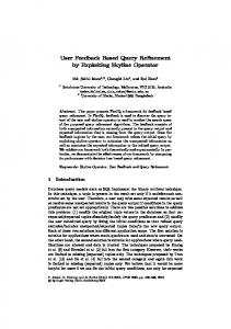
The motivation to use a set-valued transition function F and a set-valued output function H in our system description, originates from the desire to describe disturbances and other kinds of nondeterminism in a unified and concise manner. This description is also sufficiently expressive to model the plant and the controller, but unfortunately leads to subtle issues with interconnected systems. Consider e.g. the serial composition in Fig. 2, where Fi : Xi × Ui ⇒ Xi , X1 = U1 = {0}, X2 = U2 = {0, 1}, Y2 = {a, b, c}, F1 (0, 0) = {0}, H1 (0, 0) = U2 , and F2 and H2 : X2 ×U2 ⇒ Y2 are given as follows: F2 (1, 0) = F2 (0, 1) = {0}, F2 (0, 0) = F2 (1, 1) = {1}, H2 (0, 0) = H2 (1, 0) = {a}, H2 (0, 1) = {b}, and H2 (1, 1) = {c}. To recover the behavior at the terminals u1 and y2 with a system of the form (1), we let X = X1 × X2 , F : X × U1 ⇒ X and H : X × U1 ⇒ Y2 . As Y2 contains more elements than X × U1 , which can all appear in y2 , the map H must be multi-valued, which in turn implies that the following



5

property of the composed system in Fig. 2 cannot be retained: Between any two appearances of b in y2 there are an even number of a’s, and between any appearance of b and any appearance of c there are an odd number of a’s. It follows that the class of systems of the form (1) is not closed under interconnection, given the natural constraint that the state alphabet of the composed system equals the product of the state alphabets of the individual systems. To circumvent this problem we consider a slightly more general

u1

•

x1 F1 • H1 u2 • y1

x2 F2 • H2

y2

Figure 2. Serial composition of two dynamical systems of the form (1). The symbol denotes a delay.

form of system dynamics given by x(t + 1) ∈ F (x(t), v(t)), (y(t), v(t)) ∈ H(x(t), u(t)),

(2a) (2b)

where v is an internal variable. We formalize the notion of system as follows. III.1 Definition. A system is a septuple S = (X, X0 , U, V, Y, F, H),

(3)

where X, X0 , U, V and Y are nonempty sets, X0 ⊆ X, H : X ×U ⇒ Y ×V is strict, and F : X ×V ⇒ X. A quadruple (u, v, x, y) ∈ U [0;T [ × V [0;T [ × X [0;T [ × Y [0;T [ is a solution of the system (3) (on [0; T [, starting at x(0)) if T ∈ N ∪ {∞}, (2a) holds for all t ∈ [0; T − 1[, (2b) holds for all t ∈ [0; T [, and x(0) ∈ X0 . The internal variables allow us to introduce the constraint u2 = y1 imposed by the composition in Fig. 2 and recover the behavior of the serial composed system with a system of the form (3) given by X = X0 = {0, 1}, U = {0}, V = Y = {a, b, c} with F (0, a) = F (1, c) = {1}, F (1, a) = F (0, b) = {0} and H(0, 0) = {(a, a), (b, b)}, H(1, 0) = {(a, a), (c, c)}. We call the sets X, X0 , U, V , and Y the state, initial state, input, internal variable, and output alphabet, respectively. The functions F and H are, respectively, the transition function and the output function of (3). We call the system (3) (i) autonomous if U is a singleton; (ii) static if X is a singleton; (iii) Moore if the output does not depend on the input, i.e., (y, v) ∈ H(x, u) ∧ u′ ∈ U ⇒ ∃v′ (y, v ′) ∈ H(x, u′); 1 (iv) simple, if U = V , X = Y , H = id, and all states are admissible as initial states, i.e., X = X0 . We assume throughout that the plant is given by a simple system, which restricts our theory to that class of plants. B. System composition In the following, we define the serial and feedback composition of two systems. We start with the serial composition. 1

The notation ∃s A reads as “there exists s such that the statement A holds”.



6

III.2 Definition. Let Si = (Xi , Xi,0 , Ui , Vi , Yi , Fi , Hi ) be systems, i ∈ {1, 2}, and assume that Y1 ⊆ U2 . Then S1 is serial composable with S2 , and the serial composition of S1 and S2 , denoted S2 ◦ S1 , is the septuple (X12 , X1,0 × X2,0 , U1 , V12 , Y2, F12 , H12 ), where X12 = X1 × X2 , V12 = V1 × V2 , F12 : X12 × V12 ⇒ X12 and H12 : X12 × U1 ⇒ Y2 × V12 satisfy F12 (x, v) = F1 (x1 , v1 ) × F2 (x2 , v2 ), H12 (x, u1 ) = {(y2, v) | ∃y1 (y1 , v1 ) ∈ H1 (x1 , u1) ∧ (y2 , v2 ) ∈ H2 (x2 , y1 )}. We readily see that the output function H12 is strict which implies that S2 ◦ S1 is a system. We use the serial composition mainly to describe the interconnection of an input quantizer Q : U ′ ⇒ U or a state quantizer Q : X ⇒ X ′ with a system S of the form (3). We assume that Q is strict and interpret the quantizer as a static system with strict transition function. Suppose that U ′ is a non-empty set, then the serial composition S ◦ Q of Q and S is defined by S ◦ Q = (X, X0 , U ′ , V, Y, F, H ′), where H ′ : X × U ′ ⇒ Y × V takes the form H ′ (x, u′ ) = H(x, Q(u′ )). Now suppose that S is simple, then we may interpret Q : X ⇒ X ′ as a measurement map that yields a quantized version of the state of the system S. This situation is modeled by the serial composition Q ◦ S of S and Q, Q ◦ S = (X, X, U, U, X ′, F, H ′), where H ′ takes the form H ′(x, u) = Q(x) × {u}. We turn our attention to the feedback composition of two systems as illustrated in Fig. 3. III.3 Definition. Let Si = (Xi , Xi,0 , Ui , Vi , Yi , Fi , Hi ) be systems, i ∈ {1, 2}, and assume that S2 is Moore, Y2 ⊆ U1 and Y1 ⊆ U2 , and that the following condition holds: (Z) If (y2 , v2 ) ∈ H2 (x2 , y1 ), (y1 , v1 ) ∈ H1 (x1 , y2 ) and F2 (x2 , v2 ) = ∅, then F1 (x1 , v1 ) = ∅. Then S1 is feedback composable with S2 , and the closed loop composed of S1 and S2 , denoted S1 × S2 , is the septuple (X12 , X1,0 × X2,0 , {0}, V12, Y12 , F12 , H12 ), where X12 = X1 × X2 , V12 = V1 × V2 , Y12 = Y1 × Y2 , and F12 : X12 × V12 ⇒ X12 and H12 : X12 × {0} ⇒ Y12 × V12 satisfy F12 (x, v) = F1 (x1 , v1 ) × F2 (x2 , v2 ), H12 (x, 0) = {(y, v)|(y1, v1 ) ∈ H1 (x1 , y2) ∧ (y2 , v2 ) ∈ H2 (x2 , y1 )}.

F2

v2

x2

y2

H2 S2

x1

y1

H1

F1

v1

S1 Figure 3. Closed loop S1 × S2 of systems S1 and S2 according to Definition III.3, in which the system S2 is required to be Moore.



7

The requirement (Z), which has its analog in the theory developed in [2], is particularly important and will be needed later to ensure that if the concrete closed loop is non-blocking, then so is the abstract closed loop. The assumption that S2 is additionally Moore is common [34] and ensures that the closed loop does not contain a delay free cycle. We emphasize that we avoid the assumption that the controller is allowed to set the initial state of the plant, as appears e.g. in [2]. We conclude this section with a proposition that we use in several proofs throughout the paper. III.4 Proposition. Let S1 be feedback composable with S2 , and let T ∈ N ∪ {∞}. Then the closed loop S1 × S2 is an autonomous Moore system, and (0, v, x, y) is a solution of S1 × S2 on [0; T [ iff (y2 , v1 , x1 , y1 ) is a solution of S1 on [0; T [ and (y1 , v2 , x2 , y2 ) is a solution of S2 on [0; T [. Proof. We claim that H12 is strict. Indeed, assume that x ∈ X12 and a ∈ Y1 . Since H1 and H2 are both strict, there exist (y2 , b) ∈ H2 (x2 , a) and (y1 , v1 ) ∈ H1 (x1 , y2). Then there exists v2 satisfying (y2 , v2 ) ∈ H2 (x2 , y1 ) as S2 is Moore, and so (y, v) ∈ H12 (x, 0). This proves our claim. The remaining requirements in Definition III.1 are clearly satisfied, which shows that S1 × S2 is a system, and that system is autonomous, and hence, Moore. The claim on the solutions of S1 × S2 is straightforward to prove using Definitions III.1 and III.3. IV. Motivation In this section, we provide two examples that demonstrate the state information issue and the refinement complexity issue, which have led to the development of the novel notion of feedback refinement relation. Both examples show that the drawbacks do not depend on the specific refinement technique, but are intrinsic to the use of alternating (bi)simulation relations, bisimulation relations and their approximate variants. Let us consider two systems S1 and S2 and two controllers C1 and C2 , Si = (Xi , Xi , U, U, Y, Fi, Hi ), Ci = (Xc,i , Xc,i,0, Y, Vc,i, U, Fc,i , Hc,i ), in which we assume that the transition functions of the four systems are all strict, that Xi ⊆ Y , and that Hi (x, u) = {(x, u)} for all (x, u) ∈ Xi × U. We readily see that the controller Ci is feedback composable with the system Si , i ∈ {1, 2}. Subsequently, we interpret S1 as the concrete system and S2 as its abstraction. Let Q ⊆ X1 × X2 be a strict relation. Then Q is an alternating simulation relation from S1 to S2 if the following holds for every pair (x1 , x2 ) ∈ Q: (ASR) If u2 ∈ U, then there exists u1 ∈ U such that the condition ∅= 6 Q(x′1 ) ∩ F2 (x2 , u2 )

(4)

holds for every x′1 ∈ F1 (x1 , u1 ). Note that usually there is an additional condition on outputs of related states, which here would have required the notion of approximate rather than ordinary alternating simulation relation [2, Def. 9.6]. Since that subtlety is not essential to our discussion, we omit it here in favor of a clearer presentation. As already mentioned, alternating simulation relations are often used to prove the correctness of a particular abstraction-based controller design procedure. The very center of any such argument is the reproducibility of the system behavior of the concrete closed loop C1 × S1 by the abstract closed loop C2 × S2 , i.e., for every solution (0, v1 , (xc,1 , xs,1 ), y1) of C1 × S1 on Z+ there exists a solution (0, v2 , (xc,2 , xs,2 ), y2) of C2 × S2 on Z+ satisfying (xs,1 (t), xs,2 (t)) ∈ Q for all t ∈ Z+ .

(5)



8

This reproducibility property is then used to provide evidence that certain properties that the abstract closed loop C2 × S2 satisfies, actually also hold for the concrete closed loop C1 × S1 . In the first example, we show that (5) cannot hold if C1 attains state information only through Q, i.e., if C1 takes the form C1′ ◦ Q. In other words, the refined controller cannot be symbolic but requires full state information. IV.1 Example. We consider the systems S1 and S2 which we graphically illustrate by 1

S1 :

3

0 0

1

1

2

1

S2 :

3

0

1

The input and output alphabets of S1 and S2 are given by U = {0, 1} and Y = {1, 2, 3}, respectively. The transition functions should be clear from the illustration, e.g. F1 (2, 1) = {1} and F1 (1, u) = {1} for any u ∈ U. It is also easily verified that the relation Q given by Q = {(1, 1), (2, 3), (3, 3)} is an alternating simulation relation from S1 to S2 . Let the abstract controller C2 be static with Xc,2 = {0}, Vc,2 = Y , and Hc,2(0, 3) = {(0, 3)}, i.e., C2 enables exactly the control letter 0 at the abstract state 3. If the concrete controller C1 is symbolic, then, at the initial time, the sets of control letters enabled at the plant states 2 and 3 coincide. Indeed, these sets must only depend on the associated abstract states, and Q(2) = Q(3). In addition, by the symmetry of the plant S1 , we may assume without loss of generality that the control letter 0 is enabled at the initial time, so that there exists a solution (0, v1 , (xc,1, xs,1 ), y1 ) of the closed loop C1 × S1 satisfying xs,1 (0) = xs,1 (1) = 2. Then the condition (5) requires xs,2 (0) = xs,2 (1) = 3 to hold for some solution (0, v2 , (xc,2 , xs,2 ), y2) of C2 × S2 – a requirement that contradicts the dynamics of C2 × S2 . This shows that the property of reproducibility cannot be attained using a symbolic controller for the plant S1 . The crucial point with this example is that the condition (ASR) cannot be satisfied if the choice of u1 depends only on the abstract states associated with the plant state x1 , but not directly on x1 itself. In the next example we show that a static controller C2 for the abstraction S2 cannot be refined to a static controller C1 for the concrete system S1 . IV.2 Example. We consider the systems S1 and S2 with the transition functions illustrated graphically by S1 :

1

0

S2 :

2 1 4

1

0

2

0

1 3

1

4

The input alphabet and the output alphabet is given by U = {0, 1} and Y = {1, 2, 3, 4}, respectively. It is easily verified that the relation Q given by Q = {(1, 1), (2, 2), (2, 3), (4, 4)} is an alternating simulation relation from S1 to S2 . In addition, in this example the relation Q satisfies even the more restrictive requirement that u1 = u2 holds in (ASR). Suppose that the abstract controller C2 is static and enables exactly the control letters 0 and 1 at the abstract states 2 and 3, respectively. If the concrete controller C1 is static, then the set of control letters enabled at the plant state 2 does not vary with time. By the symmetry of the plant S1 , we may again assume without loss of generality that the control letter 0 is enabled at the state 2, so that there exists a solution (0, v1 , (xc,1, xs,1 ), y1 ) of the closed loop C1 × S1 satisfying xs,1 (0) = xs,1 (2) = 1. Then the condition (5) asks for xs,2 (0) = xs,2 (2) = 1 for some solution (0, v2 , (xc,2 , xs,2 ), y2) of C2 × S2 – a requirement that contradicts the dynamics of C2 ×S2 . This shows that the property of reproducibility cannot be attained using a static controller for the plant S1 despite the fact that the abstract controller



9

is static. The crucial point with this example is that the condition (4) only mandates that for each transition from x1 to x′1 in S1 there exists a state x′2 ∈ Q(x′1 ) that is a successor of x2 in S2 , but it is not required that every x′2 ∈ Q(x′1 ) succeeds x2 ; consider e.g. the case x1 = x2 = 1, x′1 = x′2 = 2. As a result, the state 1 and 4 cannot precede the state 2 and 3, respectively, in S2 , and so, implicitly, the static controller C2 has some access to the history of the solution. In contrast, at the state 2 the dynamics of S1 does not encode analogous information, which in fact could here only be provided by a controller for S1 that is dynamic rather than static. As our examples show, alternating simulation relations are not adequate for the controller refinement, whenever i) the concrete controller has merely symbolic state information and ii) the complexity of the refined controller should not exceed the complexity of the abstract controller. Moreover, we point out that in both examples the respective relation Q is not merely an alternating simulation relation according to our definition in (ASR), but also an 1-approximate bisimulation relation and 1approximate alternating bisimulation relation according to Definitions 9.5 and 9.8 in [2], respectively. Hence, the latter concepts also suffer from both issues described in this section. V. Feedback Refinement Relations In this section, we introduce feedback refinement relations as a novel means to compare systems in the context of controller synthesis, in which we focus on simple systems. A. Definition and basic properties We start by introducing the behavior of a system, where we follow the notion of infinitary completed trace semantics [35]. V.1 Definition. Let S denote the system (3). The set B(S), B(S) = {(u, y)|∃v,x,T (u, v, x, y) is a solution of S on [0; T [, and if T < ∞, then F (x(T − 1), v(T − 1)) = ∅}, (6) is called the behavior of S. Note that it often occurs that a system is non-continuable for a certain state-input pair, e.g. the terminating state of a terminating program. With our notion of system behavior, which possibly consists of finite signals as well as infinite signals, such signals are naturally included as valid elements. In our definition of system relation below, we need a notion of state dependent admissible inputs. For any simple system S of the form (3), we define the set US (x) of admissible inputs at the state x ∈ X by US (x) = {u ∈ U | F (x, u) 6= ∅} , and the image of a subset Ω ⊆ X under US is denoted US (Ω). V.2 Definition. Let S1 and S2 be simple systems, Si = (Xi , Xi , Ui , Ui , Xi , Fi , id)

(7)

for i ∈ {1, 2}, and assume that U2 ⊆ U1 . A strict relation Q ⊆ X1 × X2 is a feedback refinement relation from S1 to S2 if the following holds for all (x1 , x2 ) ∈ Q: (i) US2 (x2 ) ⊆ US1 (x1 ); (ii) u ∈ US2 (x2 ) ⇒ Q(F1 (x1 , u)) ⊆ F2 (x2 , u). The fact that Q is a feedback refinement relation from S1 to S2 will be denoted S1 4Q S2 , and we write S1 4 S2 if S1 4Q S2 holds for some Q.



10

Intuitively, and similarly to simulation relations and their variants, a feedback refinement relation from a system S1 to a system S2 associates states of S1 with states of S2 , and imposes certain conditions on the local dynamics of the systems in the associated states. However, while e.g. alternating simulation relations only require that for each input u2 admissible for S2 there exists an associated input u1 admissible for S1 [2], our definition above additionally mandates that u1 = u2 . Moreover, the definition of (approximate) alternating simulation relation requires that for each transition from x1 to x′1 in S1 there exists a state x′2 associated with x′1 and a transition from x2 to x′2 in S2 ; see condition (4). In contrast, feedback refinement relations require the existence of the latter transition for every state x′2 associated with x′1 . We next show that the relation 4 is reflexive and transitive. V.3 Proposition. Let S1 , S2 and S3 be simple systems. Then: (a) S1 4id S1 . (b) If S1 4Q S2 and S2 4R S3 , then S1 4R◦Q S3 . Proof. Suppose that Si is of the form (7), i ∈ {1, 2, 3}. The requirements in Def. V.2 are satisfied with Q = id, S1 = S2 and x1 = x2 , which proves (a). To prove (b), assume that S1 4Q S2 4R S3 . Then R ◦ Q is strict since both R and Q are so, and U3 ⊆ U1 . Let (x1 , x3 ) ∈ R ◦ Q. Then there exists x2 ∈ X2 satisfying (x1 , x2 ) ∈ Q and (x2 , x3 ) ∈ R. Thus, US3 (x3 ) ⊆ US2 (x2 ) ⊆ US1 (x1 ), and so the condition (i) in Def. V.2 is satisfied with R ◦ Q and S3 in place of Q and S2 , respectively. As for the condition (ii), additionally assume that u ∈ US3 (x3 ). Then u ∈ US2 (x2 ), and S1 4Q S2 4R S3 implies Q(F1 (x1 , u)) ⊆ F2 (x2 , u) and R(F2 (x2 , u)) ⊆ F3 (x3 , u). Then R(Q(F1 (x1 , u))) ⊆ F3 (x3 , u), and so S1 4R◦Q S3 . B. Feedback composability and behavioral inclusion In the following, we present the main result of this section. We consider three systems S1 , S2 and C and assume that C is feedback composable with S2 . We first prove that, given a feedback refinement relation Q from S1 to S2 , Q ◦ S1 and S1 are, respectively, feedback composable with C and C ◦ Q. Subsequently, we show that the behavior of the closed loops C × (Q ◦ S1 ) and (C ◦ Q) × S1 are both reproducible by the closed loop C × S2 . Even though we do not assign any particular role to the systems S1 , S2 and C, in foresight of the next section, where we use our result to develop abstraction-based solutions of general control problems, we might regard S1 , S2 and C as the plant, the abstraction and controller for the abstraction, respectively. In this context, we might assume that the state of S1 is accessible only through the measurement map Q. In that case, Q ◦ S1 actually represents the system for which we seek a controller and the behavior of B(C × (Q ◦ S1 )) is of interest. Alternatively, we may start with the premise that a controller for S1 needs to be realizable on a digital device and hence, can accept only a finite input alphabet. In that case, we may interpret Q as an input quantizer for the discrete controller C and the behavior of B((C ◦ Q) × S1 ) is of interest. In any case, we show that both behaviors are reproduced by the abstract closed loop C × S2 . In the rest of the paper, we identify {0} × (U × Y ) with U × Y in the obvious way. V.4 Theorem. Let Q be a feedback refinement relation from the system S1 to the system S2 , and assume that the system C is feedback composable with S2 . Then the following holds. (i) C is feedback composable with Q ◦ S1 , and C ◦ Q is feedback composable with S1 . (ii) B(C × (Q ◦ S1 )) ⊆ B(C × S2 ). (iii) For every (u, x1 ) ∈ B((C ◦ Q) × S1 ) there exists a map x2 such that (u, x2 ) ∈ B(C × S2 ) and (x1 (t), x2 (t)) ∈ Q for all t in the domain of x1 . Proof. By our hypotheses, S1 and S2 are simple, so we assume that these systems are of the form (7). Moreover, Q ◦ S1 = (X1 , X1 , U1 , U1 , X2 , F1 , H1′ ), (8)



11

where U2 ⊆ U1 and H1′ takes the form H1′ (x, u) = Q(x) × {u}. Let the system C be of the form C = (Xc , Xc,0, Uc , Vc , Yc , Fc , Hc ),

(9)

and observe that Yc ⊆ U1 and X2 ⊆ Uc as C is feedback composable (f.c.) with S2 . Moreover, since X1 6= ∅ and Q is strict, the serial composition C ◦ Q is well-defined, C ◦ Q = (Xc , Xc,0, X1 , Vc , Yc , Fc , Hc′ ), where Hc′ takes the form Hc′ (xc , x1 ) = Hc (xc , Q(x1 )). To prove (i), we first observe that the conditions x2 ∈ Q(x1 ), (u, v) ∈ Hc (xc , x2 ), F1 (x1 , u) = ∅

(10)

together imply Fc (xc , v) = ∅. Indeed, it follows from (10) and the requirement (i) in Definition V.2 that F2 (x2 , u) = ∅, and our claim follows as C is f.c. with S2 . This shows that C is f.c. with Q ◦ S1 . Similarly, let x1 ∈ X1 , (u, v) ∈ Hc′ (xc , x1 ) and F1 (x1 , u) = ∅. Then, by the definition of Hc′ , there exists x2 ∈ Q(x1 ) such that (u, v) ∈ Hc (xc , x2 ). Then (10) holds, and so Fc (xc , v) = ∅ as we have already shown. Hence, C ◦ Q is f.c. with S1 , which completes the proof of (i). To prove (ii), let (u, x2 ) ∈ B(C × (Q ◦ S1 )) be defined on [0; T [, T ∈ N ∪ {∞}. Then there exist maps xc , x1 and v such that (0, (v, u), (xc, x1 ), (u, x2)) is a solution of C × (Q ◦ S1 ) on [0; T [. Moreover, if additionally T < ∞, then we also have Fc (xc (T − 1), v(T − 1)) = ∅ ∨ F1 (x1 (T − 1), u(T − 1)) = ∅.

(11)

By Proposition III.4, (u, u, x1, x2 ) is a solution of Q ◦ S1 on [0; T [, and (x2 , v, xc , u) is a solution of C on [0; T [. The former fact implies the following: ∀t∈[0;T [ x2 (t) ∈ Q(x1 (t)), ∀t∈[0;T −1[ x1 (t + 1) ∈ F1 (x1 (t), u(t)).

(12) (13)

We claim that (u, u, x2, x2 ) is a solution of S2 , so that (0, (v, u), (xc, x2 ), (u, x2 )) is a solution of C × S2 by Proposition III.4. First, we observe that F2 (x2 (t), u(t)) 6= ∅ for every t ∈ [0; T − 1[. Indeed, (u(t), v(t)) ∈ Hc (xc (t), x2 (t)) for every such t since (x2 , v, xc , u) is a solution of C on [0; T [. Hence, F2 (x2 (t), u(t)) = ∅ for some t ∈ [0; T − 1[ implies Fc (xc (t), v(t)) = ∅ as C is f.c. with S2 . This is a contradiction as xc (t+1) ∈ Fc (xc (t), v(t)), so F2 (x2 (t), u(t)) 6= ∅ for every t ∈ [0; T − 1[. Consequently, u(t) ∈ US2 (x2 (t)) for all t ∈ [0; T − 1[, so (12), (13) and the requirement (ii) in Definition V.2 imply that x2 (t + 1) ∈ F2 (x2 (t), u(t)) for all t ∈ [0; T − 1[. This shows that (0, (v, u), (xc, x2 ), (u, x2 )) is a solution of C × S2 on [0; T [. Finally, we see that if T < ∞ and u(T − 1) ∈ US2 (x2 (T − 1)), then (12) and the requirement (i) in Definition V.2 together imply F1 (x1 (T − 1), u(T − 1)) 6= ∅, and in turn, (11) shows that Fc (xc (T − 1), v(T − 1)) = ∅. Thus, (u, x2 ) ∈ B(C × S2 ), which proves (ii). To prove (iii), let (u, x1 ) ∈ B((C ◦ Q) × S1 ) be defined on [0; T [, T ∈ N ∪ {∞}. Then there exist maps xc and v such that (0, (v, u), (xc, x1 ), (u, x1)) is a solution of (C ◦ Q) × S1 on [0; T [. Moreover, if additionally T < ∞, then we also have Fc (xc (T − 1), v(T − 1)) = ∅ ∨ F1 (x1 (T − 1), u(T − 1)) = ∅.

(14)

By Proposition III.4, (u, u, x1, x1 ) and (x1 , v, xc , u) is a solution of S1 and C ◦ Q, respectively. In particular, by the definition of Hc′ , there exists a map x2 : [0; T [ → X2 such that x2 (t) ∈ Q(x1 (t)) and (u(t), v(t)) ∈ Hc (xc (t), x2 (t)) for all t ∈ [0; T [. Then (x2 , v, xc , u) and (u, u, x1, x2 ) is a solution of C and Q ◦ S1 , respectively, so (0, (v, u), (xc, x1 ), (u, x2 )) is a solution of C × (Q ◦ S1 ) by Proposition III.4. We next observe that if T < ∞ and F1 (x1 (T −1), u(T −1)) 6= ∅, then (14) implies Fc (xc (T −1), v(T −1)) = ∅. This shows that (u, x2 ) ∈ B(C × (Q ◦ S1 )), and so (iii) follows from (ii).



12

Next we show, that feedback refinement relations are not only sufficient, but indeed necessary for the controller refinement as considered in this paper. V.5 Theorem. Let S1 and S2 be simple systems of the form (7), and let Q ⊆ X1 × X2 be a strict relation. If for every system C that is feedback composable with S2 follows that C is feedback composable with Q ◦ S1 and B(C × (Q ◦ S1 )) ⊆ B(C × S2 ) holds, then Q is a feedback refinement relation from S1 to S2 . Proof. In the proof we consider systems Q◦S1 of the form (8). Let C be given by ({0}, {0}, X2, {0}, U2, Fc , Hc ) with Fc (0, 0) = ∅ and Hc being strict. Then, C is feedback composable (f.c.) with S2 , and in turn, C is f.c. with Q ◦ S1 by our hypothesis. This implies U2 ⊆ U1 as required in Def. V.2. To prove that Q satisfies the condition (i) in Def. V.2, we let (x1 , x2 ) ∈ Q and u ∈ US2 (x2 ) and show that F1 (x1 , u) 6= ∅. Let C be given by ({0}, {0}, X2, X2 , U2 , Fc , Hc ) with Hc (0, x′2 ) = {(u, x′2)} for all x′2 ∈ X2 and Fc (0, x2 ) = {0} and Fc (0, x′2 ) = ∅ for x′2 ∈ X2 \ {x2 }. Then C is f.c. with S2 . In particular, the condition (Z) in Definition III.3 reduces to F2 (x2 , u) 6= ∅. Then C is also f.c. with Q ◦ S1 by our hypothesis, and here the condition (Z) implies F1 (x1 , u) 6= ∅ and the claim follows. To prove that Q satisfies the condition (ii) in Definition V.2, we choose C by ({0}, {0}, X2, X2 , U2 , Fc , Hc ) with Hc and Fc defined by: if US2 (x2 ) = ∅ we set Hc (0, x2 ) = U2 × {x2 } and Fc (0, x2 ) = ∅; otherwise Hc (0, x2 ) = US2 (x2 ) × {x2 } and Fc (0, x2 ) = {0}. With this definition of C condition (Z) holds and C is f.c. with S2 , and by our hypothesis, C is also f.c. with Q ◦ S1 . Suppose that condition (ii) does not hold, then there exist (x1 , x2 ) ∈ Q, u ∈ US2 (x2 ), x′1 ∈ F1 (x1 , u) and x′2 ∈ Q(x′1 ) such that u, u¯, x¯1 , x¯1 ) is a solution x′2 6∈ F2 (x2 , u). Let x¯1 = x1 x′1 and u¯ = uu′ with (u′ , x′2 ) ∈ Hc (0, x′2 ). Then (¯ of S1 on [0; 2[. Define x¯2 = x2 x′2 and observe that (¯ u, u¯, x ¯1 , x¯2 ) is a solution of Q ◦ S1 . Let x¯c = 00, since F2 (x2 , u) 6= ∅, we see that (u, x2 ) ∈ Hc (0, x2 ) and {0} = Fc (0, x2 ). Also (u′, x′2 ) ∈ Hc (0, x′2 ) by our choice of u′ and thus (¯ x2 , x¯2 , x¯c , u¯) is a solution of C. Hence by Proposition III.4 we see that (0, (¯ x2 , u¯), (¯ xc , x¯1 ), (¯ u, x¯2 )) is a solution of C × (Q ◦ S1 ). Consider (ˆ u, x ˆ2 ) ∈ B(C × (Q ◦ S1 )) with uˆ|[0;2[ = u¯ and xˆ2 |[0;2[ = x¯2 . Since x¯2 (1) ∈ / F2 (¯ x2 (0), u¯(0)) the sequence (0, (¯ x2 , u¯), (¯ xc , x¯2 ), (¯ u, x¯2 )) cannot be a solution of C × S2 , and so (ˆ u, xˆ2 ) ∈ / B(C × S2 ). This is a contradiction, which establishes condition (ii) in Definition V.2. VI. Symbolic Controller Synthesis In this section, we propose a controller synthesis technique based on the concept of feedback refinement relations which resolves the state information and refinement complexity issues as explained and illustrated in Sections I and IV, applies to general specifications, and produces controllers that are robust with respect to various disturbances. We follow the general three step procedure of abstractionbased synthesis outlined in Section I, where we focus on the first and third steps. Our results will be complemented by the computational method presented in Section VIII, whereas the solution of the abstract control problem – the second step of the general procedure – is beyond the scope of the present paper. Indeed, large classes of these problems can be solved efficiently using standard algorithms, e.g. [2]–[6], [17]. A. Solution of control problems We begin with the definition of the synthesis problem. VI.1 Definition. Let S denote the system (3). Given a set Z, any subset Σ ⊆ Z ∞ is called a specification on Z. A system S is said to satisfy a specification Σ on U × Y if B(S) ⊆ Σ. Given a specification Σ on U × Y , the system C solves the control problem (S, Σ) if C is feedback composable with S and the closed loop C × S satisfies Σ. It is clear that we can use linear temporal logic (LTL) to define a specification for a given system S. Indeed, suppose that we are given a finite set P of atomic propositions, a labeling function



13

L : U × Y ⇒ P and an LTL formula ϕ defined over P, see e.g. [24, Chapter 5]. Then we can formulate the control problem (S, Σ) to enforce the formula ϕ on S using the specification Σ = {(u, y) ∈ (U × Y )Z+ | L ◦ (u, y) satisfies ϕ}. Our notion of specification is not limited to LTL, e.g. “y(t) = 1 holds for all even t ∈ Z+ ” is not expressible in LTL [24, Remark 5.43], but is a valid specification in our framework. We are now going to solve control problems using Theorem V.4. As we have already discussed, the concrete control problem (S1 , Σ1 ) will not be solved directly. Instead, we will consider an auxiliary problem for the abstraction (“abstract control problem”), whose solution will induce a solution of the concrete problem. VI.2 Definition. Let S1 and S2 be simple systems of the form (7), let Σ1 be a specification on U1 ×X1 , and let Q ⊆ X1 ×X2 be a strict relation. A specification Σ2 on U2 ×X2 is called an abstract specification associated with S1 , S2 , Q and Σ1 , if the following condition holds. If (u, x2 ) ∈ Σ2 , where x2 and u are defined on [0; T [ for some T ∈ N ∪ {∞}, and if x1 : [0; T [ → X1 satisfies (x1 (t), x2 (t)) ∈ Q for all t ∈ [0; T [, then (u, x1 ) ∈ Σ1 . For the sake of simplicity, we write (S1 , Σ1 ) 4Q (S2 , Σ2 ) whenever S1 4Q S2 and Σ2 is an abstract specification associated with S1 , S2 , Q and Σ1 . The result presented below shows how to use a solution of the abstract control problem to arrive at a solution of the concrete control problem, resulting in the closed loop in Fig. 1. VI.3 Theorem. If (S1 , Σ1 ) 4Q (S2 , Σ2 ) and the abstract controller C solves the control problem (S2 , Σ2 ), then the refined controller C ◦ Q solves the control problem (S1 , Σ1 ). Proof. As C solves (S2 , Σ2 ), C is feedback composable with S2 , and hence, C ◦ Q is feedback composable with S1 by Theorem V.4. It remains to show that B((C ◦ Q) × S1 ) ⊆ Σ1 . So, let (u, x1 ) ∈ B((C ◦ Q) × S1 ) be arbitrary and invoke Theorem V.4 again to see that there exists a map x2 such that (u, x2 ) ∈ B(C × S2 ) and (x1 (t), x2 (t)) ∈ Q for all t in the domain of x2 . Then (u, x2 ) ∈ Σ2 since C solves (S2 , Σ2 ), and the definition of the abstract specification Σ2 shows that (u, x1 ) ∈ Σ1 . B. Uncertainties and disturbances We next show that it is an easy task in our framework to synthesize controllers that are robust with respect to various disturbances including plant uncertainties, input disturbances and measurement errors. In particular, we demonstrate that the synthesis of a robust controller can be reduced to the solution of an auxiliary, unperturbed control problem. Let us consider the closed loop illustrated in Fig. 4 consisting of a plant given by a simple system S1 of the form (7), the perturbation maps Pi , given by strict set-valued maps with non-empty domains

and a strict quantizer

ˆ1 , P1 : Uˆ1 ⇒ U1 , P2 : X1 ⇒ X P3 : Uˆ1 ⇒ Y1 , P4 : X1 ⇒ Y2 ,

(15)

ˆ 1 ⇒ X2 . Q: X

(16)

We seek to synthesize a controller given as a system C = (Xc , Xc,0, X2 , Vc , Uˆ1 , Fc , Hc ),

(17)

to robustly enforce a given specification Σ1 on Y1 × Y2 . The behavior of the closed loop in Fig. 4 is defined as the set of all sequences (y1 , y2 ) ∈ (Y1 ×Y2 )[0;T [ , T ∈ N ∪ {∞}, for which there exist a solution (u, u, x, x) of S1 on [0; T [ and a solution (uc , vc , xc , yc ) of C on [0; T [ that satisfy the following two conditions:



14

(i) For all t ∈ [0; T [ we have u(t) ∈ P1 (yc (t)), y1 (t) ∈ P3 (yc (t)),

uc (t) ∈ Q(P2 (x(t))), y2 (t) ∈ P4 (x(t)).

(18)

(ii) If T < ∞, then F1 (x(T − 1), u(T − 1)) = ∅, or Fc (xc (T − 1), vc (T − 1)) = ∅. u

S1

yc P3

P4

y2

P2

P1

y1

x

(19)

Q C

uc

Figure 4. Various perturbations in the closed loop.

It is straightforward to observe, that the perturbations maps P1 and P2 may be used to model input disturbances and measurement errors, respectively. We assume that the uncertainties of the dynamics of S1 have already been modeled by the set-valued transition function F1 . The controller C and the quantizer Q, which will usually be discrete, are not subject to any additional perturbations either. The maps P3 and P4 are useful in the presence of output disturbances. For example, the plant S1 might represent a sampled variant of a continuous-time control system and the specification of the desired behavior is naturally formulated in continuous time, rather than in discrete time. In that context, one can use P3 and P4 to “robustify” the specification like in [36] such that properties of the sampled behavior carry over to the continuous-time behavior. ˆ 1 on Uˆ1 × X1 , we call Σ ˆ 1 a robust specification of Σ1 Given some specifications Σ1 on Y1 × Y2 and Σ ˆ w.r.t. P3 and P4 if for the functions (yc , x, y1 , y2 ) ∈ (U1 × X1 × Y1 × Y2 )[0;T [ , T ∈ N ∪ {∞}, we have that ˆ 1 and ∀t∈[0;T [ y1 (t) ∈ P3 (yc (t)), y2 (t) ∈ P4 (x(t)) (yc , x) ∈ Σ implies (y1 , y2 ) ∈ Σ1 . In the following result, we present sufficient conditions for a controller C to robustly enforce a given specification Σ1 on the perturbed closed loop illustrated in Fig. 4, in terms of the auxiliary simple system Sˆ1 , ˆ1 , X1 , Fˆ1 , id), Sˆ1 = (X1 , X1 , Uˆ1 , U Fˆ1 (x, u) = F1 (x, P1 (u)),

(20)

ˆ 1 of Σ1 . We show in the subsequent corollary, which follows together with a robust specification Σ immediately by Theorem VI.3, how to use an abstraction (S2 , Σ2 ) to synthesize such a controller C. VI.4 Theorem. Consider a simple system S1 , perturbation maps Pi , i ∈ [1; 4], a strict quantizer Q, and a controller C as illustrated in Fig. 4 and respectively defined in (7), (15), (16) and (17), and ˆ 1 ) be an auxiliary control assume that F1 is strict. Let Σ1 be a specification on Y1 × Y2 . Let (Sˆ1 , Σ ˆ 1 is a robust specification of Σ1 w.r.t. P3 problem, where Sˆ1 follows from S1 according to (20) and Σ and P4 .



15

ˆ with Q ˆ = Q ◦ P2 , solves the control problem (Sˆ1 , Σ ˆ 1 ), then the behavior of the perturbed If C ◦ Q, closed loop in Fig. 4 is a subset of Σ1 . ˆ is feedback composable with Sˆ1 . Using Definition III.3, Proof. Our assumptions imply that C ◦ Q Proposition III.4, the strictness of F1 , and the properties (18)-(19), it is straightforward to show that ˆ Sˆ1 ) (y1 , y2 ) is an element of the behavior of the closed loop in Fig. 4 iff there exists (yc , x) ∈ B((C ◦ Q)× satisfying y1 (t) ∈ P3 (yc (t)) and y2 (t) ∈ P4 (x(t)) for all t. Consequently, if (y1 , y2) is an element of ˆ 1 satisfying y1 (t) ∈ P3 (yc (t)) and the behavior of the closed loop in Fig. 4, then there exist (yc , x) ∈ Σ ˆ 1. y2 (t) ∈ P4 (x(t)) for all t, and so (y1 , y2 ) ∈ Σ1 by the definition of Σ VI.5 Corollary. In the context of Theorem VI.4, if C solves an abstract control problem (S2 , Σ2 ) with ˆ 1 ) 4 ˆ (S2 , Σ2 ), where X2 is the state space of S2 , then the behavior of the closed loop in Fig. 4 (Sˆ1 , Σ Q is a subset of Σ1 . In the following example we demonstrate that it is crucial to account for the measurement errors P2 ˆ = Q◦P2 , as opposed to accounting for those type of disturbances in terms of the auxiliary quantizer Q ˆ1 , Uˆ1 , X1 , F˜1 , id) with F˜1 given by in terms of an alternative auxiliary system S˜1 = (X1 , X1 , U F˜1 (x1 , u) = P2 (F1 (x1 , P1 (u))). (21) VI.6 Example. We consider the simple system S1 of the form (7) with the transition function illustrated graphically a

1

c

{0, 1}

0

b {0, 1} 0

1 d

{0, 1}

The state and input alphabet are given by X1 = {a, b, c, d} and U1 = {0, 1}, respectively. Suppose we are given the specification Σ1 on U1 × X1 defined implicitly by (u, x) ∈ Σ1 iff d is in the image of x. Let us consider the quantizer Q = id and the perturbation maps P1 = P3 = P4 = id and P2 defined by P2 (a) = {a}, P2 (b) = P2 (c) = {b, c} and P2 (d) = {d}. Let the auxiliary system S˜1 coincide with S1 except the transition function is given by F˜1 (x, u) = P2 (F1 (x, u)). The controller C ◦ Q, with C given as static system with strict transition function and output map Hc : {0} × X1 ⇒ U1 × X1 defined by Hc (0, a) = Hc (0, d) = U1 × {a}, Hc (0, b) = {(1, a)}, Hc (0, c) = {(0, a)} solves the control problem (S˜1 , Σ1 ). However, (u, x) = (0, a), (1, c), (1, c), (1, c), . . . is an element of the behavior of the closed loop according to Fig. 4 and yet violates the specification Σ1 .

As the example demonstrates, we cannot rely on the auxiliary system with transition function (21) to synthesize a robust controller but we need a quantizer that is robust with respect to disturbances. ˆ with Q ˆ = Q ◦ P2 solves the auxiliary control That is essentially expressed by requiring that C ◦ Q ˆ 1 ). Intuitively, we require that the controller C “works” with any quantizer symbol problem (Sˆ1 , Σ x2 ∈ Q(P2 (x1 )) no matter how the disturbance P2 is acting on the state x1 . Note that in Example VI.6, ˆ 1 ) (which in this case equals the controller C ◦ (id ◦P2 ) does not solve the control problem (Sˆ1 , Σ (S1 , Σ1 )). Finally, we would like to mention that in the context of control systems, any symbolic controller synthesis procedure that is based on a deterministic quantizer is bound to be non-robust. Indeed, consider the context of Theorem VI.4 and suppose that X1 = Rn , X2 is a partition of X1 and let P2 (x1 ) equal the closed Euclidean ball with radius ε ≥ 0 centered at x1 . Let us consider the deterministic ˆ = Q ◦ P2 is deterministic only in the degenerate case ε = 0. quantizer Q = ∈ . Then Q VII. Canonical Feedback Refinement Relations In this section, we show that the set membership relation ∈, together with an abstraction whose state alphabet is a cover of the concrete state alphabet is canonical. A cover of a set X is a set of



16

subsets of X whose union equals X. We show that (S1 , Σ1 ) 4Q (S3 , Σ3 ) implies that there exist (S2 , Σ2 ), with X2 being a cover of X1 by non-empty subsets, together with a relation R such that the following holds: (S1 , Σ1 ) 4∈ (S2 , Σ2 ) 4R (S3 , Σ3 ). This implies that if we can solve the concrete control problem (S1 , Σ1 ) using some abstract control problem (S3 , Σ3 ), then we can equally use an abstract control problem (S2 , Σ2 ) with X2 being to a cover of X1 by non-empty subsets. Moreover, (S2 , Σ2 ) can be derived from the problem (S3 , Σ3 ) and the quantizer Q alone and is otherwise independent of (S1 , Σ1 ). A. Canonical abstractions VII.1 Proposition. Let S1 and S2 be simple systems of the form (7), in which X2 is a cover of X1 by non-empty subsets and U2 ⊆ U1 . Then S1 4∈ S2 iff the following conditions hold. (i) x ∈ Ω ∈ X2 implies US2 (Ω) ⊆ US1 (x). (ii) If Ω, Ω′ ∈ X2 , u ∈ US2 (Ω) and Ω′ ∩ F1 (Ω, u) 6= ∅, then Ω′ ∈ F2 (Ω, u). The above result, whose straightforward proof we omit, will be used in our proof of the canonicity result, Theorem VII.2. It additionally indicates constructive methods to compute a canonical abstraction S2 of a plant S1 if the abstract state space X2 and the input alphabet U2 ⊆ U1 are given. From condition (ii) it follows that, if Ω ∈ X2 , u ∈ U2 and F1 (x, u) 6= ∅ for every x ∈ Ω, then we may either choose F2 (Ω, u) to be empty, which is of course not desirable2 , or ensure that the latter set contains every cell Ω′ that intersects the attainable set F1 (Ω, u) of the cell Ω under the control letter u. This can be achieved by numerically over-approximating attainable sets, for which many algorithms are available, see e.g. [7] and Section VIII. On the other hand, condition (i) requires that F2 (Ω, u) is empty whenever F1 (x, u) is so for some x ∈ Ω. This raises the question of how to detect the phenomenon of blocking of the dynamics of the plant. If the transition function F1 is explicitly given, we assume that its description directly facilitates the detection of blocking. In the case that the plant represents a sampled system, so that F1 is the time-τ -map of some continuous-time control system, blocking can usually be detected in the course of over-approximating attainable sets. For example, if an over-approximation W of the attainable set F1 (Ω, u) is computed using interval arithmetic, and if F1 (x, u) = ∅ for some x ∈ Ω, then W will be unbounded, e.g. [37, Chapter II.3], which is easily detected. B. Canonicity result Before we state and prove the canonicity result, we introduce a technical condition that we impose on the feedback refinement relation Q from (S1 , Σ1 ) to (S3 , Σ3 ), i.e., (C) if ∅ = 6 Q−1 (x) = Q−1 (˜ x), ∅ = 6 Q−1 (x′ ) = Q−1 (˜ x′ ), x˜′ ∈ F3 (˜ x, u), and u ∈ US3 (x), then x′ ∈ F3 (x, u). We point out that condition (C) is not an essential restriction and it actually holds for a great variety of abstractions and relations. For example, it automatically holds if the abstraction S3 is defined as a quotient system [2, Definition 4.17]. In that case, the elements of X3 correspond to the equivalence classes of an equivalence relation on X1 . Therefore, we have that Q−1 (x) = Q−1 (˜ x) implies x = x˜ and condition (C) is trivially satisfied. Similarly, relations that are based on level n sets of simulation functions V : X1 × X3 → pR+ with X1 , X3 ⊆ R , see e.g. [18], for popular choices of simulation functions like V (x1 , x3 ) = (x1 − x3 )⊤ P (x1 − x3 ) with P being a positive definite 2 One should always choose F2 (Ω, u) 6= ∅, since it enlarges the set of control letters available to any abstract controller and thereby facilitates the solution of the abstract control problem.



17

matrix, where x⊤ denotes the transpose of x, satisfy (C). In this case, the relation is given by Q = {(x1 , x3 ) ∈ X1 × X3 | V (x1 , x3 ) ≤ ε} and again Q−1 (x) = Q−1 (˜ x) implies x = x˜ and we conclude that (C) holds. Lastly, the condition (C) also holds, for the case that Q is given and the abstraction S3 is computed using a deterministic algorithm to over-approximate attainable sets. This is immediate from the following reformulation of the condition (ii) in Definition V.2: If x2 , x′2 ∈ X2 , u ∈ US2 (x2 ), and Q−1 (x′2 ) ∩ F1 (Q−1 (x2 ), u) 6= ∅, then x′2 ∈ F2 (x2 , u). VII.2 Theorem. Let (S3 , Σ3 ) be a control problem, in which S3 is simple and of the form (7). Let X1 be any set, and assume that Q : X1 ⇒ X3 satisfies the condition (C). Then there exist a simple system S2 of the form (7), a relation R ⊆ X2 × X3 and a specification Σ2 on U2 × X2 such that the following holds. (∗) If (S1 , Σ1 ) 4Q (S3 , Σ3 ) and the system S1 has state space X1 , then (S1 , Σ1 ) 4∈ (S2 , Σ2 ) 4R (S3 , Σ3 ) and X2 is a cover of X1 by non-empty subsets. Proof. We will prove that (∗) holds for the following choices of S2 , R and Σ2 : X2 = {Ω | ∅ = 6 Ω = Q−1 (x) ∧ x ∈ X3 }, R(Ω) = {x ∈ X3 | Ω = Q−1 (x)}, U2 = U3 , F2 (Ω, u) = R−1 (F3 (R(Ω), u)), and (u, Ω) ∈ (U2 × X2 )∞ is an element of Σ2 iff there exists (u, x3 ) ∈ Σ3 satisfying (Ω(t), x3 (t)) ∈ R for all t in the domain of u. To establish (∗), assume that (S1 , Σ1 ) 4Q (S3 , Σ3 ). Then Q is strict, which already proves our claim on X2 , and S1 is simple, and so we can assume that S1 takes the form (7). To prove S1 4∈ S2 , we first notice that the condition (i) in Proposition VII.1 is satisfied. Indeed, let x1 ∈ Ω ∈ X2 and u ∈ US2 (Ω). By our choice of F2 and R, there exists x3 satisfying (x1 , x3 ) ∈ Q and u ∈ US3 (x3 ). Then u ∈ US1 (x1 ) by Def. V.2 applied to S1 4Q S3 . To establish the condition (ii) in Prop. VII.1, we let Ω, Ω′ ∈ X2 and u ∈ US2 (Ω) and assume that Ω′ ∩ F1 (Ω, u) 6= ∅. By the latter fact there exist x1 ∈ Ω and x′1 ∈ Ω′ ∩ F1 (x1 , u), and u ∈ US2 (Ω) implies that there exists x3 such that Ω = Q−1 (x3 ) and u ∈ US3 (x3 ). We pick x′3 satisfying Ω′ = Q−1 (x′3 ). Then (x1 , x3 ), (x′1 , x′3 ) ∈ Q, and so S1 4Q S3 implies x′3 ∈ Q(x′1 ) ⊆ F3 (x3 , u). Hence, Ω′ ∈ F2 (Ω, u) by our choice of F2 . This proves S1 4∈ S2 . To prove S2 4R S3 , let (Ω, x3 ) ∈ R and u ∈ US3 (x3 ) and pick any x1 ∈ Ω. Then (x1 , x3 ) ∈ Q by our choice of R, and using S1 4Q S3 we obtain u ∈ US1 (x1 ). The latter fact implies that there exists x′1 ∈ F1 (x1 , u), and using S1 4Q S3 again we see that Q(x′1 ) ⊆ F3 (x3 , u). Since Q is strict we may pick x′3 ∈ Q(x′1 ). Then R−1 (x′3 ) 6= ∅, and hence, u ∈ US2 (Ω) by the definition of F2 , which proves the condition (i) in Definition V.2. To prove the condition (ii) in that definition, let (Ω, x3 ) ∈ R, u ∈ US3 (x3 ) and Ω′ ∈ F2 (Ω, u). Then Ω′ ∈ R−1 (F3 (Ω, u)), so there exist x˜3 and x˜′3 ∈ F3 (˜ x3 , u) satisfying Ω = Q−1 (˜ x3 ) and Ω′ = Q−1 (˜ x′3 ). Then condition (C) implies x′3 ∈ F3 (x3 , u), and in turn, R(Ω′ ) ⊆ F3 (x3 , u). To complete the proof, we notice that, by the definition of Σ2 , Σ3 is an abstract specification associated with S2 , S3 , R and Σ2 , which shows (S2 , Σ2 ) 4R (S3 , Σ3 ). Finally, to prove (S1 , Σ1 ) 4∈ (S2 , Σ2 ), let (u, Ω) ∈ Σ1 , assume that u is defined on [0; T [, and let x1 : [0; T [ → X1 satisfy x1 (t) ∈ Ω(t) for all t ∈ [0; T [. Then, by the definition of Σ2 , there exists (u, x3 ) ∈ Σ3 such that R(Ω(t)) = {x3 (t)} for all t ∈ [0; T [. The latter condition implies (x1 (t), x3 (t)) ∈ Q, and (S1 , Σ1 ) 4Q (S3 , Σ3 ) implies (u, x1 ) ∈ Σ1 . VIII. Computation of Abstractions for Perturbed Sampled Control Systems In the previous section we have seen that the computation of abstractions basically reduces to the over-approximation of attainable sets of the plant. A large number of over-approximation methods have been proposed which apply to different classes of systems, e.g. [2], [7], [38]–[40]. In this section, we present an approach to over-approximate attainable sets of continuous-time perturbed control systems, based on a matrix-valued Lipschitz inequality.



18

A. The sampled system Let us consider a perturbed control system of the form x˙ ∈ f (x, u) + W

(22)

with f : Rn × U → Rn , U ⊆ Rm and W ⊆ Rn . We assume throughout this section that U is non-empty, W contains the origin, and that f (·, u) is locally Lipschitz for all u ∈ U. We use the set W to represent various uncertainties in the dynamics of the control system (22). For τ ∈ R+ and an interval I ⊆ [0, τ ], a solution of (22) on I with (constant) input u ∈ U is defined ˙ ∈ f (ξ(t), u) + W for almost every as an absolutely continuous function ξ : I → Rn that satisfies ξ(t) (a.e.) t ∈ I. We say that ξ is continuable to [0, τ ] if there exists a solution ξ¯ of (22) on [0, τ ] with ¯ I = ξ. input u ∈ U such that ξ| We formulate a sampled variant of (22) as system as follows. VIII.1 Definition. Let S1 be a simple system of the form (7), and let τ > 0. We say that S1 is the sampled system associated with the control system (22) and the sampling time τ , if X1 = Rn , U1 = U and the following holds: x1 ∈ F1 (x0 , u) iff there exist a solution ξ of (22) on [0, τ ] with input u satisfying ξ(0) = x0 and ξ(τ ) = x1 . In the sequel, ϕ denotes the general solution of the unperturbed system associated with (22) for constant inputs. That is, if x0 ∈ Rn , u ∈ U, and f (·, u) is locally Lipschitz, then ϕ(·, x0 , u) is the unique non-continuable solution of the initial value problem x˙ = f (x, u), x(0) = x0 [37]. Similar to other approaches [14], [15] to over-approximate attainable sets that are known for unperturbed systems, our computation of attainable sets of the perturbed system is based on an estimate of the distance of neighboring solutions of (22). VIII.2 Definition. Consider the sets K ⊆ Rn , U ′ ⊆ U and the sampling time τ > 0. A map β : Rn+ × U ′ → Rn+ is a growth bound on K, U ′ associated with τ and (22) if the following conditions hold: (i) β(r, u) ≥ β(r ′ , u) whenever r ≥ r ′ and u ∈ U ′ , (ii) [0, τ ] × K × U ′ ⊆ dom ϕ and if ξ is a solution of (22) on [0, τ ] with input u ∈ U ′ and ξ(0), p ∈ K then |ξ(τ ) − ϕ(τ, p, u)| ≤ β(|ξ(0) − p|, u) (23) holds component-wise. Let us emphasize some distinct features of the estimate (23). First of all, we formulate the inequality (23) component-wise, which allows to bound the difference of neighboring solutions for each state coordinate independently. Second, β is a local estimate, i.e., we require (23) to hold only for initial states in K. Moreover, β is allowed to depend on the input, but these inputs are assumed to be constant, and we do not bound the effect of different inputs on the distance of the solutions. All those properties contribute to more accurate over-approximations of the attainable sets. This, in turn, leads to less conservative abstractions; see our example in Section IX-A. Note that it is also immediate to account for extensions like time varying inputs and using different sampling times. B. The abstraction We continue with the construction of an abstraction S2 of the sampled system S1 . The state alphabet X2 of the abstraction is defined as a cover of the state alphabet X1 where the elements of the cover X2 are non-empty, closed hyper-intervals, i.e., every element x2 ∈ X2 takes the form Ja, bK = Rn ∩ ([a1 , b1 ] × · · · × [an , bn ]) for some a, b ∈ (R ∪ {±∞})n , a ≤ b.



19

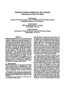
Our notion of hyper-intervals allows for unbounded cells in X2 . Nevertheless, in the computation ¯ 2 ⊆ X2 of compact cells. We interpret the cells in X ¯2 of the abstraction S2 , we work with a subset X as the “real” quantizer symbols, and the remaining ones, as overflow symbols, see [7, Sect. III.A]. ¯ 2 ⊆ X2 and a VIII.3 Definition. Consider two simple systems S1 and S2 of the form (7), a set X n n function β : R+ × U2 → R+ . Given τ > 0, suppose that S1 is the sampled system associated with (22) ¯ 2 and β, if and sampling time τ . We call S2 an abstraction of S1 based on X ¯ 2 is compact; (i) X2 is a cover of X1 by non-empty, closed hyper-intervals and every element x2 ∈ X (ii) U2 ⊆ U1 ; ¯ 2 , x′ ∈ X2 and u ∈ U2 we have (iii) for x2 ∈ X 2 (ϕ(τ, c, u) + J−r ′ , r ′ K) ∩ x′2 6= ∅ ⇒ x′2 ∈ F2 (x2 , u),

(24)

where Ja, bK = x2 , c = b+a , r = b−a and r ′ = β(r, u); 2 2 ¯ 2 , u ∈ U2 . (iv) F2 (x2 , u) = ∅ whenever x2 ∈ X2 \ X Note that the implicit definition of the transition function F2 according to (iii) in Definition VIII.3 ¯ 2 , then Ja′ , b′ K ∈ X2 has to be an is equivalently expressible as follows. Let u ∈ U2 and Ja, bK ∈ X element of F2 (Ja, bK , u) if a′ − r ′ ≤ ϕ(τ, c, u) ≤ b′ + r ′ holds, where c, r and r ′ are as in Definition VIII.3. We illustrate the transition function F2 (x2 , u) of an abstraction in Fig. 5. x2 r2

c r1

X2

F2 (x2 , u) r2′

r1′

ϕ(τ, c, u)

Figure 5. Illustration of the transition function of an abstraction.

¯ 2 ⊆ X2 , and VIII.4 Theorem. Consider two simple systems S1 and S2 of the form (7) and a set X let τ > 0. Suppose that S1 is the sampled system associated with (22) and sampling time τ . Let β be ¯2 a growth bound on ∪x2 ∈X¯2 x2 , U2 associated with τ and (22). If S2 is an abstraction of S1 based on X and β, then S1 4∈ S2 . ¯ 2 by Proof. To verify the condition (i) in Proposition VII.1 first note that US2 (x2 ) = ∅ if x2 ∈ X2 \ X ¯ our assumption on S2 . On the other hand, if x1 ∈ x2 ∈ X2 , then U2 ⊆ US1 (x1 ) by our assumption on β, so the condition (i) in Proposition VII.1 is satisfied. To verify the requirement (ii) in Proposition ¯ 2 by our assumption on S2 , so VII.1, assume that x2 , x′2 ∈ X2 and u ∈ US2 (x2 ). Then x2 ∈ X x2 = Jc − r, c + rK for some c, r. Moreover, if additionally x1 ∈ x2 and x′2 ∩ F1 (x1 , u) 6= ∅, then by Definition VIII.1 there exists a solution ξ : [0, τ ] → Rn of the system (22) with input u satisfying ξ(0) = x1 and ξ(τ ) ∈ x′2 . It follows that |ξ(0) − c| ≤ r, and hence, |ξ(τ ) − ϕ(τ, c, u)| ≤ r ′ . Then (24) implies that x′2 ∈ F2 (x2 , u). An application of Proposition VII.1 completes the proof. As seen from the above proof, the set ϕ(τ, c, u) + J−r ′ , r ′K in (24) over-approximates the attainable set F1 (Ja, bK , u). The approximation error, which greatly influences the accuracy of the abstraction, can be reduced by working with smaller cells Ja, bK. However, the accuracy can also be ¯ 2 by compact hyperimproved without rediscretizing the state space X1 , by covering cells Ja, bK ∈ X intervals γi + J−ρi , ρi K with ρi < r, i ∈ I, and then using, in place of the premise in (24), the test ∃i∈I (ϕ(τ, γi , u) + J−β(ρi , u), β(ρi , u)K) ∩ x′2 6= ∅.



20

C. A growth bound In this subsection we present a specific growth bound for the case that f is continuously differentiable in its first argument and the perturbations are given by W = J−w, wK for some w ∈ Rn+ . In the following proposition, we use Dj fi to denote the partial derivative with respect to the jth component of the first argument of fi . VIII.5 Theorem. Let τ > 0 and let f , U and W be as in (22) with W = J−w, wK for some w ∈ Rn+ . Let U ′ ⊆ U and assume in addition that f (·, u) is continuously differentiable for every u ∈ U ′ . Furthermore, let K ⊆ K ′ ⊆ Rn with K ′ being convex, so that for any u ∈ U ′ , any τ ′ ∈ [0, τ ] and any solution ξ on [0, τ ′ ] of (22) with input u and ξ(0) ∈ K, we have ξ(t) ∈ K ′ for all t ∈ [0, τ ′ ]. Lastly, let the parametrized matrix L : U ′ → Rn×n satisfy ( Dj fi (x, u), if i = j, Li,j (u) ≥ |Dj fi (x, u)|, otherwise for all x ∈ K ′ and all u ∈ U ′ . Then any ξ as above is continuable to [0, τ ], and the map β given by Z τ L(u)τ β(r, u) = e r+ eL(u)s w ds 0

′

is a growth bound on K, U associated with τ and (22).

Theorem VIII.5 can be applied quite easily for obtaining growth bounds. Firstly, the computation of an a priori enclosure K ′ to solutions of (22) is standard, e.g. [41] and the references therein. Secondly, the parametrized matrix L requires bounding partial derivatives on K ′ . Such bounds can be computed in an automated way using, e.g., interval arithmetic [42]. Finally, given L, the evaluation of the expression for β is straightforward. We emphasize, however, that Theorem VIII.5 provides only one of several methods to over-approximate attainable sets. Any over-approximation method can be used to compute abstractions based on feedback refinement relations. Having a growth bound at hand, the application of Theorem VIII.4 becomes a routine task. Examples are presented in the next section. For the proof of Theorem VIII.5 we need the following auxiliary result, which appears in [43] without proof. VIII.6 Lemma. Let τ > 0 and A ⊆ Rn . Let ξi : [0, τ ] → A, i ∈ {1, 2}, be two perturbed solutions of a dynamical system with continuous right hand side f : Rn → Rn , i.e., the maps ξi are absolutely continuous and satisfy |ξ˙i (t) − f (ξi (t))| ≤ wi (t) for a.e. t ∈ [0, τ ] , where wi : [0, τ ] → Rn+ , i ∈ {1, 2}, are integrable. Consider a matrix L ∈ Rn×n with Li,j ≥ 0 for i 6= j and suppose that for all x, y ∈ A we have Xn xi ≥ yi ⇒ fi (x) − fi (y) ≤ Li,j |xj − yj |. (25) j=1

Let ρ : [0, τ ] →

Rn+

be absolutely continuous and satisfying

ρ(t) ˙ = Lρ(t) + w1 (t) + w2 (t) for a.e. t ∈ [0, τ ]. Then |ξ1 (0) − ξ2 (0)| ≤ ρ(0) implies |ξ1 (t) − ξ2 (t)| ≤ ρ(t) for every t ∈ [0, τ ]. ρ(t) + w1 (t) + Proof. Let ρ˜ : [0, τ ] → Rn+ be absolutely continuous such that ρ˜(0) = ρ(0) and ρ˜′ (t) = L˜ w2 (t) + ε for some ε ∈ (R+ \ {0})n and a.e. t ∈ [0, τ ]. We shall prove that |ξ1 (t) − ξ2 (t)| ≤ ρ˜(t)

(26)



21

holds for all t ∈ [0, τ ], so that the lemma follows from a limit argument. To this end, denote the function ξ1 − ξ2 − ρ˜ on [0, τ ] by z and let t0 = sup{t ∈ [0, τ ] | ∀s∈[0,t] z(s) ≤ 0}. Then t0 ≥ 0 as |ξ1 (0) − ξ2 (0)| ≤ ρ(0), and since we can interchange the roles of ξ1 and ξ2 if necessary, we may assume without loss of generality that (26) holds for all t ∈ [0, t0 ]. It remains to show that t0 = τ . Assume that t0 < τ . Using (26), a continuity argument shows that we may choose t2 ∈ ]t0 , τ ] and i ∈ [1; n] such that zi (t2 ) > 0, zi (t0 ) = 0 and Xn Xn Li,j |ξ1,j (t) − ξ2,j (t)| (27) Li,j ρ˜j (t) ≥ εi + j=1

j=1

for all t ∈ [t0 , t2 ]. Define t1 = sup{t ∈ [t0 , t2 ] | zi (t) ≤ 0} and note that zi (t1 ) = 0 as zi is continuous. The inequality zi′ (t) ≤ fi (ξ1 (t)) −fi (ξ2 (t)) + w1,i (t) + w2,i (t) − ρ˜′i (t) for a.e. t ∈ [t1 , t2 ] and the definition of ρ˜ then imply that Z t2 n X zi (t2 ) ≤ fi (ξ1 (t)) − fi (ξ2 (t)) − Li,j ρ˜j (t) − εi dt. t1

j=1

Thus, zi (t2 ) ≤ 0 by (27) and (25). This contradicts our choice of t2 , and so t0 = τ .

Proof of Theorem VIII.5. Fix p ∈ K, u ∈ U ′ and note that β(r, u) ≥ β(r ′ , u) if r ≥ r ′ as all entries of eL(u)τ are non-negative [44, Th. 7.7]. Next, we show that condition (ii) in Definition VIII.2 holds. In order to apply Lemma VIII.6 we shall establish (25) for K ′ , f (·, u) and L(u) in place of A, f and L. Indeed, by the P mean value theorem, there exists z ∈ {x + t(y − x)|t ∈ [0, 1]} such that fi (x, u) − fi (y, u) = nj=1 Dj fi (z, u)(xj − yj ). Hence, by the definition of L, we obtain (25). Now, let ξ be a solution on [0, τ ] of (22) with input u such that ξ(0) ∈ K. By Filippov’s Lemma [45], ˙ = f (ξ(t), u) + s(t) for a.e. t ∈ [0, τ ]. So, there exists an integrable map s : [0, τ ] → W such that ξ(t) ′ apply Lemma VIII.6 to f (·, u), K , ϕ(·, p, u), ξ, 0, w and L(u) in place of f , A, ξ1 , ξ2 , w1 , w2 and L, respectively, to obtain |ξ(τ ) − ϕ(τ, p, u)| ≤ β(|ξ(0) − p|, u). Finally, suppose there exists ξ : [0, τ ′ ] → K ′ as in the statement of the theorem that is not continuable to [0, τ ]. Then, there exist t0 ∈ [0, τ ] and a solution ξ¯: [0, t0 [ → Rn of (22) with input u such that ¯ [0,τ ′ ] = ξ and ξ(t) ¯ becomes unbounded as t ∈ [0, t0 [ approaches t0 [46]. On the other hand, applying ξ| ¯ [0,t] , ξ(0), w, |f (ξ(0), u)|, L(u) and t in place of f , A, ξ1 , ξ2 , w1 , w2 , L Lemma VIII.6 to f (·, u), K ′ , ξ| ¯ − ξ(0)| is uniformly bounded for t ∈ [0, t0 [, which is a contradiction. and τ we conclude that |ξ(t) D. The Case of Periodic Dynamics Occasionally we will have to consider continuous-time control systems of the form (22) whose dynamics are periodic, i.e., f (ξ + p, ·) = f (ξ, ·) for some period p ∈ Rn \ {0} and all ξ ∈ Rn . Our result below shows how to exploit periodicity to obtain abstractions that are finite and yet are capable of reproducing solutions that are unbounded in the direction of the period. This is useful, e.g. when one of the components of the state represents an angle and the number of full loops is potentially unbounded; see Section IX-A for an example. VIII.7 Theorem. Let p1 , . . . , pℓ ∈ Rn , ℓ ∈ N, be such that f in (22) satisfies f (x + pi , u) = f (x, u) for all i ∈ [1; ℓ], x ∈ Rn and u ∈ U. Consider systems S1 and S2 of the form (7), where U2 ⊆ U1 and S1 is the sampled system associated o with (22) and sampling time τ > 0. Define the map π : X1 ⇒ X1 n Pℓ ℓ by π(x) = x + i=1 ki pi k ∈ Z , and let R be a set of non-empty subsets of X1 such that X2 = {π(Ω) | Ω ∈ R} and X2 is a cover of X1 . Then S1 4∈ S2 iff the following conditions hold: (a) x ∈ Ω ∈ R implies US2 (π(Ω)) ⊆ US1 (x). (b) If Ω, Ω′ ∈ R, u ∈ US2 (π(Ω)) and π(Ω′ ) ∩ F1 (Ω, u) 6= ∅, then π(Ω′ ) ∈ F2 (π(Ω), u). Obviously, the transition function F2 of the system S2 can be computed by over-approximating attainable sets F1 (Ω, u) as detailed in Sections VII-A, VIII-B and VIII-C, and by verifying the


condition (Ω′ + k ∈ Zℓ .

Pℓ


i=1 ki pi )

22

∩ F1 (Ω, u) 6= ∅, for Ω, Ω′ ∈ R with Ω being compact, and finitely many

ℓ Proof. First Pℓ observe that F1 (x, u) + hk|pi = F1 (x + hk|pi , u) for all k ∈ Z , x ∈ Xℓ1 and u ∈ U1 , where hk|pi = i=1 ki pi . Then US1 (x + hk|pi) = US1 (x) for all x ∈ X1 and all k ∈ Z , which shows that the condition (i) in Proposition VII.1 is equivalent to (a). We shall show that the condition (ii) is equivalent to (b), which proves the theorem. If Ω, Ω′ ∈ R, u ∈ US2 (π(Ω)) and π(Ω′ ) ∩ F1 (Ω, u) 6= ∅, then π(Ω), π(Ω′ ) ∈ X2 and Ω ⊆ π(Ω), and so (ii) shows that π(Ω′ ) ∈ F2 (π(Ω), u). Conversely, if Ω, Ω′ ∈ X2 , u ∈ US2 (Ω) and Ω′ ∩ F1 (Ω, u) 6= ∅, then there exist Ω0 , Ω′0 ∈ R satisfying Ω = π(Ω0 ) and Ω′ = π(Ω′0 ). Hence, π(Ω′0 ) ∩ (hk|pi + F1 (Ω0 , u)) 6= ∅ for some k ∈ Zℓ , and since π(Ω′0 ) = π(Ω′0 ) + hk|pi we have π(Ω′0 ) ∩ F1 (Ω0 , u) 6= ∅. Then (b) shows that Ω′ ∈ F2 (Ω, u), which completes the proof.

IX. Examples In this section, we demonstrate the practicality of our approach on control problems for nonlinear plants. A. A path planning problem for an autonomous vehicle We consider an autonomous vehicle whose dynamics we assume to be given by the bicycle model in [47, Ch. 2.4]. More concretely, the dynamics of the system are of the form (22), where f : R3 × U → R3 is given by   u1 cos(α + x3 ) cos(α)−1 f (x, (u1 , u2)) =  u1 sin(α + x3 ) cos(α)−1  u1 tan(u2 )

with U = [−1, 1] × [−1, 1] and α = arctan(tan(u2)/2). Here, (x1 , x2 ) is the position and x3 is the orientation of the vehicle in the 2-dimensional plane. The control inputs u1 and u2 are the rear wheel velocity and the steering angle. Perturbations are not acting on the system dynamics, i.e., W = {(0, 0, 0)}. The concrete control problem is formulated with respect to the sampled system S1 associated with (22) and sampling time τ = 0.3. The control objective is to enforce a certain patrolling behavior on the vehicle which is situated in a maze; see Fig. 6. Specifically, the vehicle, whose initial state is A1,0 = {(0.4, 0.4, 0)}, should patrol infinitely often between the target regions A1,r1 = [0, 0.5] × [0, 0.5] × R and A1,r2 = (9, 0, 0) + A1,r1 , while avoiding the obstacles A1,a . The third component of A1,a equals R. We formalize our concrete control problem through the pair (S1 , Σ1 ) with the specification Σ1 defined as {(u, x) ∈ (U1 × X1 )Z+ | x(0) ∈ A1,0 ⇒ ∀t∈Z+ (x(t) ∈ / A1,a ∧ ∀i∈{1,2} ∃t′ ∈[t;∞[ x(t′ ) ∈ A1,ri )},

(28)

where U1 = U and X1 = R3 . To solve (S1 , Σ1 ) we solve an abstract control problem (S2 , Σ2 ) as detailed below. As f possesses the period p = (0, 0, 2π) we construct a canonical abstraction S2 of the form (7) using Theorem VIII.7, where R consist of the shifted copies of the hyper-interval 1 1 1 1 π π − 10 , 10 × − 10 , 10 × − 35 , 35 ,

2 2 whose centers form the set 10 [0; 50] × 10 [0; 50] × 2π [−17; 17], and of the hyper-intervals {x ∈ R3 | 35 xj ≥ 10.1}, {x ∈ R3 | xj ≤ −0.1}, j ∈ {1, 2}. Set U2 = {0, ±0.3, ±0.6, ±0.9} × {0, ±0.3, ±0.6, ±0.9}, and let X2 be as in Theorem VIII.7. The transition function F2 is computed according to the remark following Theorem VIII.7, in which F2 (x2 , u) = ∅ if (x2 , u) ∈ X2 × U2 , x2 ∩ A1,a 6= ∅. The required growth bound β on R3 , U2 associated with τ and (22) is obtained using Theorem VIII.5. In



23

p particular, β(r, u) = eL(u)τ r, where L is given by L1,3 (u1, u2 ) = L2,3 (u1 , u2 ) = |u1 tan2 (u2 )/4 + 1|, and Li,j (u1 , u2 ) = 0 for (i, j) ∈ / {(1, 3), (2, 3)}. The computation of F2 takes 2.25 seconds (Intel Core i7 2.9 GHz) resulting in an abstraction having 37266181 transitions. To construct the abstract specification Σ2 we let A2,0 = {x2 ∈ X2 | x2 ∩ A1,0 6= ∅}, A2,ri = {x2 ∈ X2 | x2 ⊆ A1,ri }, i ∈ {1, 2} and A2,a = {x2 ∈ X2 | x2 ∩ A1,a 6= ∅}; see Fig. 6. We define Σ2 by (28), where we substitute U1 , X1 , A1,0 , A1,r1 , A1,r2 , A1,a with U2 , X2 , A2,0 , A2,r1 , A2,r2 , A2,a , respectively. It is straightforward to verify that Σ2 is an abstract specification associated with S1 , S2 , ∈ and Σ1 . The abstract problem (S2 , Σ2 ) can be solved using the algorithm in [6, Fig. 1], which simplifies here to two rather than three nested fixed-point iterations since for our problem the general reactivity (1) 6 F2 (x, u) ⊆ A}. specification in [6] reduces to νZ.∩i∈{1,2} µY.( Y ∪(A2,ri ∩ Z)), where A = {x ∈ X2 | ∃u∈U2 ∅ = We actually use a Dijkstra-like algorithm [48] for the inner fixed-point to successfully solve (S2 , Σ2 ) within 0.54 seconds. The solution is refined to a solution of (S1 , Σ1 ) by adding a static quantizer; see Theorem VI.3. A similar problem with considerably less complex specification is solved in [14], where the run times in seconds are 13509 (abstraction) and 535 (synthesis) on Intel Core 2 Duo 2.4 GHz. We would like to discuss two of the advantages of the growth bounds we have introduced in Section VIII. As we already mentioned, β bounds each component of neighboring solutions separately, which can be directly seen by the formula β(r, u) = r + r3 · L1,3 (u1 , u2 ) ·(τ, τ, 0)⊤. This distinguishes β from an estimate based on a norm. Moreover, β depends on the input, which is crucial for the present example. Indeed, the function e(sup L)τ r, where sup L ∈ R3×3 is given by (sup L)i,j = supu∈U2 Li,j (u), is also a growth bound on R3 , U2 associated with τ and (22), which leads to an abstraction with 43288873 transitions. However, due to the poor approximation quality of this growth bound we obtain an unsolvable abstract control problem. B. An aircraft landing maneuver We consider an aircraft DC9-30 whose dynamics we model according to [49]. We use x1 , x2 , x3 to denote the state variables, which respectively correspond to the velocity, the flight path angle and the altitude of the aircraft. The input alphabet is given by U = [0, 160 · 103 ] × [0◦ , 10◦ ] and represents the thrust of the engines (in Newton) and the angle of attack. The dynamics are given by f : R3 ×U → R3 ,   1 (u cos u − D(u , x ) − mg sin x ) 1 2 2 1 2 m 1 (u1 sin u2 + L(u2 , x1 ) − mg cos x2 ) , f (x, u) =  mx 1 x1 sin x2

where D(u2 , x1 ) = (2.7 + 3.08 · (1.25 + 4.2 · u2 )2 ) · x21 , L(u2 , x1 ) = (68.6 · (1.25 + 4.2 · u2 )) · x21 and mg = 60 · 103 · 9.81 account for the drag, lift and gravity, respectively [49]. We consider the input disturbance P1 : U ⇒ U given by P1 (u) = (u+[−5 · 103 , 5 · 103 ]×[−0.25◦ , 0.25◦ ])∩ 1 U and measurement errors of the form P2 : R3 ⇒ R3 given by P2 (x) = x + 20 [−0.25, 0.25] × 1 1 ◦ ◦ [−0.05 , 0.05 ]× 20 [−1, 1]. We do not consider any further disturbances, i.e., we let W = {(0, 0, 0)}, 20 P3 = id, and P4 = id. The concrete control problem is formulated with respect to the sampled system S1 = (X1 , X1 , U1 , U1 , X1 , F1 , i associated with (22) and the sampling time τ = 0.25. We aim at steering the aircraft from an altitude of 55 meters close to the ground with an appropriate total and horizontal touchdown velocity. More formally, the specification Σ1 is given by Σ1 = (u, x) ∈ (U1 × X1 )Z+ | x(0) ∈ A0 ⇒ (29) (∃s∈Z+ x(s) ∈ Ar ∧ ∀t∈[0;s[ x(t) ∈ / Aa ) ,

where I = [−3◦ , 0◦ ], A0 = [80, 82] × [−2◦ , −1◦ ] × {55},

Aa = R3 \ ([58, 83] × I × [0, 56]), Ar = ([63, 75] × I × [0, 2.5]) ∩ {x ∈ R3 |x1 sin x2 ≥ −0.91}.



24

10

5

0 0

5

10

Figure 6. Projection of the states of S1 and S2 to R2 × {0}. The sets A1,a and A1,r1 , A1,r2 are indicated in dark blue and in red, respectively. The states in A2,a and A2,r1 ,A2,r2 are indicated in blue and in light red, respectively. A closed-loop trajectory of the concrete control problem is shown evolving from A1,r1 to A1,r2 in the blue part and vice versa in the green part.

As detailed in Section VI-B, the perturbed control problem is solved through an auxiliary unperturbed control problem. To begin with, define the simple system Sˆ1 by (20) with Uˆ1 = U. Next, let X be a cover of R3 formed by subdividing R3 \ Aa into 210 · 210 · 210 hyper-intervals, and suitable unbounded ¯ 2 be the subset of compact elements of X2 hyper-intervals. Define X2 = {P2−1 (Ω) | Ω ∈ X} and let X ˆ that do not intersect Aa . Define the abstraction for S1 as the simple system S2 given by (7), where U2 = {0, 32000} × U ′ , U ′ contains precisely 10 inputs equally spaced in [0◦ , 8◦ ]. We apply Theorem VIII.5 with w = M(5000, 0.25◦)⊤ ≤ (0.108, 0.002, 0)⊤ and a suitable a priori enclosure K ′ to obtain 2×3 a growth bound, where M ∈ R+ satisfies Mi,j ≥ |Dj,2fi (x, u)| for all x ∈ K ′ and u ∈ P1 (U2 ). Here, Dj,2 fi stands for the partial derivative with respect to the jth component of the second argument of fi . Note that w accounts for the perturbation P1 . Then, we use Theorem VIII.4 to compute F2 such that Sˆ1 4∈ S2 . The computation takes 674 seconds resulting in an abstraction with about 9.38 · 109 transitions (Intel Xeon E5 3.1 GHz). To construct the abstract specification Σ2 for S2 we let A2,0 = {x2 ∈ X2 | x2 ∩ A1,0 6= ∅}, A2,a = {x2 ∈ X2 | x2 ∩ A1,a 6= ∅}, A2,r = {x2 ∈ X2 | x2 ⊆ A1,r } and define the specification Σ2 by (29) with U2 , X2 , A2,0 , A2,r , A2,a in place of U1 , X1 , A0 , Ar , Aa . It is easy to verify that Σ2 is an abstract specification associated with Sˆ1 , S2 , ∈ and Σ1 . Note that Σ2 (as well as Σ1 ) is a particular instance of a reach-avoid specification. Using a standard technique [48], the abstract control problem (S2 , Σ2 ) is successfully solved within 26 seconds. By Corollary VI.5 the behavior of the perturbed closed loop is a subset of Σ1 . See Fig. 7. We proceed to make some comments on solving perturbed control problems. At first, Theorem VIII.5 allows to deal with time-varying input perturbations, when the theorem is applied as in this example. Second, accounting for measurement errors only requires inflating the cells that would have



25

been used if measurement errors were not present. To conclude, perturbed control problems can be solved in our framework by using canonical abstractions. x3 50 40 30 20 10 0

5

10

15

t

Figure 7. Time evolution of the altitude of the aircraft in the closed loop. The aircraft pitch u2 + x2 is indicated for 8 instants of time.

X. Conclusions We have presented a novel approach to abstraction-based controller synthesis which builds on the concept of feedback refinement relation introduced in the present paper. Our framework incorporates several distinct features. Foremost, the designed controllers require quantized (or symbolic) state information only and are connected to the plant via a static quantizer, which is particularly important for any practical implementation of the controller. Our work permits the synthesis of robust correctby-design controllers in the presence of various uncertainties and disturbances, and more generally, applies to a broader class of synthesis problems than previous research addressing the state information and refinement complexity issues as explained and illustrated in Sections I and IV. Moreover, we do not assume that the controller is able to set the initial state of the plant, which is also important in the context of practical control systems. We have additionally identified a class of canonical abstractions, and have presented a method to compute such abstractions for perturbed nonlinear control systems. We utilized numerical examples to demonstrate the applicability and efficiency of our synthesis framework. We emphasize, however, that the computational effort is still expected to grow rapidly with the dimension of the state space of the plant, a problem that is shared by all grid based methods for the computation of abstractions. Acknowledgment The authors thank M. Mazo (Delft), T. Moor (Erlangen), P. Tabuada (Los Angeles) and M. Zamani (M¨ unchen) for fruitful discussions about this research. References [1] S. Palnitkar, Verilog HDL: A Guide to Digital Design and Synthesis, 2nd ed. Prentice Hall PTR, 2003. [2] P. Tabuada, Verification and control of hybrid systems. New York: Springer, 2009. [3] E. A. Emerson and E. M. Clarke, “Using branching time temporal logic to synthesize synchronization skeletons,” Sci. Comput. Programming, vol. 2, no. 3, pp. 241–266, 1982. [4] A. Pnueli and R. Rosner, “On the synthesis of an asynchronous reactive module,” in Proc. 16th Intl. Coll. Automata, languages and programming, Stresa, Italy, Jul. 11-15, 1989, ser. Lect. Notes Computer Science. Springer, Berlin, 1989, vol. 372, pp. 652–671. [5] M. Y. Vardi, “An automata-theoretic approach to fair realizability and synthesis,” in Proc. 7th Intl. Conf. Computer Aided Verification (CAV), Li`ege, Belgium, Jul. 3-5, 1995, ser. Lect. Notes Computer Science, vol. 939. London, UK: Springer-Verlag, 1995, pp. 267–278. [6] R. Bloem, B. Jobstmann, N. Piterman, A. Pnueli, and Y. Sa’ar, “Synthesis of reactive(1) designs,” J. Comput. System Sci., vol. 78, no. 3, pp. 911–938, 2012.



26

[7] G. Reißig, “Computing abstractions of nonlinear systems,” IEEE Trans. Automat. Control, vol. 56, no. 11, pp. 2583–2598, Nov. 2011, DOI:10.1109/TAC.2011.2118950, arXiv:0910.2187. [8] L. Gr¨ une and O. Junge, “Approximately optimal nonlinear stabilization with preservation of the Lyapunov function property,” in Proc. 46th IEEE Conf. Decision and Control (CDC), New Orleans, LA, U.S.A., 2007. New York: IEEE, 2007, pp. 702–707. [9] G. Kreisselmeier and T. Birkh¨ olzer, “Numerical nonlinear regulator design,” IEEE Trans. Automat. Control, vol. 39, no. 1, pp. 33–46, 1994. [10] A. Girard, “Low-complexity quantized switching controllers using approximate bisimulation,” Nonlinear Anal. Hybrid Syst., vol. 10, pp. 34–44, 2013. [11] B. Yordanov, J. Tumova, I. Cerna, J. Barnat, and C. Belta, “Temporal logic control of discrete-time piecewise affine systems,” IEEE Trans. Automat. Control, vol. 57, no. 6, pp. 1491–1504, 2012. [12] E. Dallal, A. Colombo, D. Del Vecchio, and S. Lafortune, “Supervisory control for collision avoidance in vehicular networks with imperfect measurements,” in Proc. 52th IEEE Conf. Decision and Control (CDC), Florence, Italy, 10-13 Dec. 2013. New York: IEEE, 2013, pp. 6298–6303. [13] J. Liu and N. Ozay, “Abstraction, discretization, and robustness in temporal logic control of dynamical systems,” in Proc. 17th Intl. Conf. Hybrid Systems: Computation and Control (HSCC), Berlin, Germany, Apr. 15-17, 2014, 2014, pp. 293–302. [14] M. Zamani, G. Pola, M. Mazo, Jr., and P. Tabuada, “Symbolic models for nonlinear control systems without stability assumptions,” IEEE Trans. Automat. Control, vol. 57, no. 7, pp. 1804–1809, 2012. [15] M. Rungger and O. Stursberg, “On-the-fly model abstraction for controller synthesis,” in American Control Conference (ACC), 2012, pp. 2645–2650. [16] X. D. Koutsoukos, P. J. Antsaklis, J. A. Stiver, and M. D. Lemmon, “Supervisory control of hybrid systems,” Proc. IEEE, vol. 88, no. 7, pp. 1026–1049, Jul. 2000. [17] G. Reissig and M. Rungger, “Abstraction-based solution of optimal stopping problems under uncertainty,” in Proc. IEEE Conf. Decision and Control (CDC), Florence, Italy, 10-13 Dec. 2013. New York: IEEE, 2013, pp. 3190–3196, DOI:10.1109/CDC.2013.6760370. [18] A. Girard and G. J. Pappas, “Approximation metrics for discrete and continuous systems,” IEEE Trans. Automat. Control, vol. 52, no. 5, pp. 782–798, 2007. [19] T. Moor, K. Schmidt, and T. Wittmann, “Abstraction-based control for not necessarily closed behaviours,” in Proc. 18th IFAC World Congress, Milano, Italy, Aug. 28 - Sep. 2, 2011. IFAC, 2011, pp. 6988–6993. [20] A. Girard, “Approximately bisimilar abstractions of incrementally stable finite or infinite dimensional systems,” in Proc. IEEE Conf. Decision and Control (CDC), Los Angeles, CA, U.S.A., 15-17 Dec. 2014. New York: IEEE, 2014, pp. 824–829. [21] G. Reissig and M. Rungger, “Feedback refinement relations for symbolic controller synthesis,” in Proc. IEEE Conf. Decision and Control (CDC), Los Angeles, CA, U.S.A., 15-17 Dec. 2014. New York: IEEE, 2014, pp. 88–94. [Online]. Available: http://dx.doi.org/10.1109/CDC.2014.7039364 [22] L. Benvenuti, A. Ferrari, E. Mazzi, and A. Sangiovanni-Vincentelli, “Contract-based design for computation and verification of a closed-loop hybrid system,” in Proc. 11th Intl. Conf. Hybrid Systems: Computation and Control (HSCC), St. Louis, USA, Apr. 22-24, 2008, ser. Lect. Notes Computer Science, vol. 4981. Springer, 2008, pp. 58–71. [23] S. Tripakis, B. Lickly, T. A. Henzinger, and E. A. Lee, “A theory of synchronous relational interfaces,” ACM Trans. Program. Lang. Syst., vol. 33, no. 4, p. 14, 2011. [24] C. Baier and J.-P. Katoen, Principles of model checking. MIT Press, Cambridge, MA, 2008. [25] E. D. Sontag, Mathematical control theory, 2nd ed., ser. Texts in Applied Mathematics. New York: Springer-Verlag, 1998, vol. 6. [26] P. E. Caines and Y.-J. Wei, “Hierarchical hybrid control systems: a lattice-theoretic formulation,” IEEE Trans. Automat. Control, vol. 43, no. 4, pp. 501–508, 1998. [27] G. E. Fainekos, H. Kress-Gazit, and G. J. Pappas, “Temporal logic motion planning for mobile robots,” in Proc. IEEE Intl. Conf. Robotics and Automation (ICRA), Barcelona, Spain, 18-22 Apr. 2005, 2005, pp. 2032–2037. [28] L. C. G. J. M. Habets, P. J. Collins, and J. H. van Schuppen, “Reachability and control synthesis for piecewise-affine hybrid systems on simplices,” IEEE Trans. Automat. Control, vol. 51, no. 6, pp. 938–948, 2006. [29] L. C. G. J. M. Habets, P. J. Collins, and J. H. van Schuppen, “Control to facet by piecewise-affine output feedback,” IEEE Trans. Automat. Control, vol. 57, no. 11, pp. 2831–2843, 2012. [30] H. Kress-Gazit, T. Wongpiromsarn, and U. Topcu, “Correct, reactive, high-level robot control,” IEEE Robotics and Automation Magazine, vol. 18, no. 3, pp. 65–74, 2011. [31] M. K. Helwa and M. E. Broucke, “Monotonic reach control on polytopes,” IEEE Trans. Automat. Control, vol. 58, no. 10, pp. 2704–2709, 2013. [32] M. K. Helwa and P. E. Caines, “On the construction of in-block controllable covers of nonlinear systems on polytopes,” in Proc. IEEE Conf. Decision and Control (CDC), Osaka, Japan, 15-18 Dec. 2015. New York: IEEE, 2015, pp. 276–281. [33] R. T. Rockafellar and R. J.-B. Wets, Variational analysis, ser. Grundlehren der Mathematischen Wissenschaften. Berlin: Springer-Verlag, 1998, vol. 317, 3rd corr printing 2009. [34] M. Vidyasagar, Input-output analysis of large-scale interconnected systems, ser. Lect. Notes Control Inform. Sciences. Berlin: Springer-Verlag, 1981, vol. 29. [35] R. J. van Glabbeek, “The linear time–branching time spectrum. I. The semantics of concrete, sequential processes,” in Handbook of process algebra, J. A. Bergstra, A. Ponse, and S. A. Smolka, Eds. Amsterdam: North-Holland, 2001, pp. 3–99. [36] G. E. Fainekos, A. Girard, H. Kress-Gazit, and G. J. Pappas, “Temporal logic motion planning for dynamic robots,” Automatica J. IFAC, vol. 45, no. 2, pp. 343–352, 2009.



27

[37] P. Hartman, Ordinary differential equations, ser. Classics in Applied Mathematics. Philadelphia, PA, U.S.A.: Society for Industrial and Applied Mathematics (SIAM), 2002, vol. 38. [38] O. Junge, “Rigorous discretization of subdivision techniques,” in International Conference on Differential Equations, Vol. 1, 2 (Berlin, 1999). World Sci. Publ., River Edge, NJ, 2000, pp. 916–918. [39] G. Osipenko, Dynamical systems, graphs, and algorithms, ser. Lecture Notes in Mathematics. Berlin: Springer-Verlag, 2007, vol. 1889. [40] A. Weber and G. Reissig, “Classical and strong convexity of sublevel sets and application to attainable sets of nonlinear systems,” SIAM J. Control Optim., vol. 52, no. 5, pp. 2857–2876, 2014, DOI:10.1137/130945983, arXiv:1311.4989. [Online]. Available: http://dx.doi.org/10.1137/130945983 [41] N. S. Nedialkov, K. R. Jackson, and G. F. Corliss, “Validated solutions of initial value problems for ordinary differential equations,” Appl. Math. Comput., vol. 105, no. 1, pp. 21–68, 1999. [42] R. E. Moore, Interval analysis. Englewood Cliffs, N.J.: Prentice-Hall Inc., 1966. [43] W. Walter, Differential and integral inequalities, ser. Translated from the German by Lisa Rosenblatt and Lawrence Shampine. Ergebnisse der Mathematik und ihrer Grenzgebiete, Band 55. New York: Springer-Verlag, 1970. [44] T. Kato, A short introduction to perturbation theory for linear operators. New York: Springer-Verlag, 1982. [45] A. F. Filippov, “On certain questions in the theory of optimal control,” J. SIAM Control Ser. A, vol. 1, pp. 76–84, 1962. [46] A. F. Filippov, Differential equations with discontinuous righthand sides, ser. Mathematics and its Applications (Soviet Series). Kluwer Academic Publishers Group, Dordrecht, 1988, vol. 18, translated from the Russian. Astr¨ om and R. M. Murray, Feedback systems. Princeton University Press, Princeton, NJ, 2008. [47] K. J. ˚ [48] G. Gallo, G. Longo, S. Pallottino, and S. Nguyen, “Directed hypergraphs and applications,” Discrete Appl. Math., vol. 42, no. 2-3, pp. 177–201, 1993, combinatorial structures and algorithms. [49] I. Mitchell, A. Bayen, and C. Tomlin, “Validating a hamilton-jacobi approximation to hybrid system reachable sets,” in Proc. 4th Intl. Conf. Hybrid Systems: Computation and Control (HSCC), Rome, Italy, Mar. 28-30, 2001, ser. Lect. Notes Computer Science, M. Di Benedetto and A. Sangiovanni-Vincentelli, Eds., vol. 2034. Springer, 2001, pp. 418–432.

Feedback Refinement Relationsfor the Synthesis of Symbolic ... - arXiv

Feedback Refinement Relationsfor the Synthesis of Symbolic ... - arXiv

Suggest Documents

Approaching Symbolic Parallelization by Synthesis of ... - arXiv

Approaching Symbolic Parallelization by Synthesis of ... - arXiv

User Feedback Based Query Refinement by

Ranking Refinement via Relevance Feedback in Geographic ...

Symbolic Partition Refinement with Dynamic Balancing of Time and ...

Formal refinement of extended state machines - arXiv

A symbolic algorithm for the synthesis of bounded ... - Semantic Scholar

Refinement of MIMO Limited-Feedback using Second ... - Google Sites

Photographic Image Synthesis with Cascaded Refinement Networks

Symbolic Computation of the Roots of any Polynomial with ... - arXiv

A symbolic algorithm for the synthesis of bounded

On the Use of Symbolic Analyzers in Circuit Synthesis

Symbolic Computation of the Roots of any Polynomial with ... - arXiv

Unbeast: Symbolic Bounded Synthesis⋆ - Reactive Systems Group

Sonification of Probabilistic Feedback through Granular Synthesis

Sonification of Probabilistic Feedback through Granular Synthesis

Ontology Verbalization using Semantic-Refinement - arXiv

Piecewise rotations: symbolic dynamics arXiv ...

Fast Matrix Multiplication and Symbolic Computation - arXiv

Symbolic Manipulators Affect Mathematical Mindsets - arXiv

Query Refinement and User Relevance Feedback for Contextualized ...

Feedback-Control of Photoresponsive Fluid Interfaces - arXiv

synthesis and characterization of - arXiv

The Impact of Galactic Feedback on the CGM - arXiv