execution-time measurements. The controllers may also communicate feedforward mode-change infor- mation to the scheduler. As an example, we con-.
39th IEEE Conference on Decision and Control, Sydney, Australia, December 2000
Feedback Scheduling of Control Tasks Anton Cervin and Johan Eker Department of Automatic Control Lund Institute of Technology Box 118, SE-221 00 Lund, Sweden {anton,johane}@control.lth.se
Abstract The paper presents a feedback scheduling mechanism in the context of co-design of the scheduler and the control tasks. We are particularly interested in controllers where the execution time may change abruptly between different modes, such as in hybrid controllers. The proposed solution attempts to keep the CPU utilization at a high level, avoid overload, and distribute the computing resources evenly among the tasks. The feedback scheduler is implemented as a periodic or sporadic task that assigns sampling periods to the controllers based on execution-time measurements. The controllers may also communicate feedforward mode-change information to the scheduler. As an example, we consider hybrid control of a set of double-tank processes. The system is evaluated, from both scheduling and control performance perspectives, by co-simulation of controllers, scheduler, and tanks.
1. Introduction There is currently a trend towards more flexible realtime control systems. By combining scheduling theory and control theory, it is possible to achieve higher resource utilization and better control performance. To achieve the best results, co-design of the scheduler and the controllers is necessary. This research area is only beginning to emerge, and there is still a lot of theoretical and practical work to be done, both in the control community and in the real-time community. Control tasks are generally viewed by the scheduling community as hard real-time tasks with fixed sampling periods and known WCETs. Upon closer inspection, neither of these assumptions need necessarily be true. For instance, many control algorithms are quite robust against variations in sampling period and response time. Controllers can be designed to switch between different modes with different execution times and perhaps also different sampling in-
tervals. It is also possible to consider control systems that are able to do a trade-off between the available computation time and the control loop performance. As an example throughout this paper, we study the problem of scheduling a set of hybrid-control tasks. Such tasks are good examples of tasks that do not really meet the assumptions commonly made in the scheduling theory. A hybrid controller switches between different modes, which may have very different execution-time characteristics. Utilizing only worst-case execution-time (WCET) estimates in the scheduling design can result in very low resource utilization, slow sampling, and low control performance. On the other hand, if instead, for instance, average-case execution-time estimates are used in the scheduling design, the CPU may experience transient overloads during run-time. This, again, can result in low control performance, and even temporary shut-down of the controllers. In this work, we present a feedback scheduler for control tasks that attempts to keep the CPU utilization at a high level, avoid overload, and distribute the computing resources evenly among the tasks. While we want to keep the number of missed deadlines as low as possible, control performance is our primary objective. Thus, control tasks, in our view, fall in a category somewhere between hard and soft real-time tasks. The known-WCET assumption is relaxed by the use of feedback from execution-time measurements. We also introduce feedforward to further improve the regulation of the utilization. The structure of the feedback scheduler is shown in Figure 1. A set of control tasks generate jobs that are fed to the run-time dispatcher. The scheduler gets feedback information about the actual execution time, ci, of the jobs (it is assumed that this information can be provided by real-time operating system). It also gets feedforward information from control tasks that are about to switch mode. This way, the scheduler can proact rather than react to sudden changes in the workload. The scheduler tries to keep
mode changes Usp Scheduler
Figure 1
{ Ti }
Tasks
jobs
Dispatcher
ci , U
The feedback scheduling structure.
utilization, U , as close as possible to the utilization setpoint, Usp. This is done by manipulating the sampling periods, { Ti}. The choice of utilization setpoint depends on the scheduling policy of the dispatcher, and on the sensitivity of the controllers to missed deadlines. Notice that the well-known, guaranteed utilization bounds of 100% for earliest-deadline-first (EDF) scheduling and 69% for fixed-priority scheduling are not valid in this context, since the assumptions about known, fixed WCETs and fixed periods are violated. The calculated task periods should reflect the relative importance of the different control tasks. One possibility is to assign nominal sampling periods to the controllers off-line. The feedback scheduler can then do linear rescaling of the task periods to achieve the desired utilization. The controllers are informed of the new sampling periods and may adjust their parameters if necessary. Other possibilities could include on-line optimization of a control performance criterion over the task periods, subject to the utilization constraint. The feedback scheduler is in the end also implemented as a periodic or sporadic task that consumes computing resources. There is a fundamental trade-off between the time that should be spent doing scheduling, and the time left over for control computations. 1.1 Related Work The related work falls into three categories. The first one is the field of integrated control system and realtime system design. In [Seto et al., 1996], sampling period selection for a set of control tasks is considered. The performance of a task is given as function of its sampling frequency, and an optimization problem is solved to find a set of optimal task periods. Co-design of real-time control systems is also considered in [Ryu et al., 1997], where the performance parameters are expressed as functions of the sampling periods and the input-output latencies. [Shin and Meissner, 1999] deals with on-line rescaling and relocation of control tasks in a multi-processor system. A simulator for co-design is introduced in [Eker and Cervin, 1999]. It facilitates co-simulation of control task execution, scheduling, and continuous plant dynamics.
The second area of related work is on quality-ofservice (QoS) aware real-time software, where a system’s resource allocation is adjusted on-line in order to maximize the performance in some respect. In [Li and Nahrstedt, 1998] a general framework is proposed for controlling the application requests for system resources using the amount of allocated resources for feedback. It is shown that a PID controller can be used to bound the resource usage in a stable and fair way. A resource allocation scheme called Q-RAM is presented in [Rajkumar et al., 1997]. Several tasks are competing for finite resources, and each task is associated with a utility value, which is a function of the assigned resources. The system distributes the resources between the tasks to maximize the total utility of the system. In [Abdelzaher et al., 1997] a QoS renegotiation scheme is proposed as a way to allow graceful degradation in cases of overload, failures or violation of pre-runtime assumptions. The mechanism permits clients to express, in their service requests, a range of QoS levels they can accept from the provider, and the perceived utility of receiving service at each of these levels. The third area relates to the wealth of flexible scheduling algorithms available. An interesting alternative to linear task rescaling is given in [Buttazzo et al., 1998], where an elastic task model for periodic tasks is presented. The relative sensitivity of tasks to rescaling are expressed in terms of elasticity coefficients. Schedulability analysis of the system under EDF scheduling is given. Closely related to our work, [Stankovic et al., 1999] presents a scheduling algorithm that explicitly uses feedback. A PID controller regulates the deadline miss-ratio for a set of soft real-time tasks with varying execution times, by adjusting their requested CPU utilization. It is assumed that tasks can change their CPU consumption by executing different versions of the same algorithm. An admission controller is used to accommodate larger changes in the workload. 1.2 Outline The rest of the paper is outlined as follows. Section 2 describes a hybrid controller for a double-tank process. Section 3 applies the feedback scheduling principle to a system with three hybrid controllers. The design and implementation are discussed and simulation results are given. Finally, Section 4 contains the conclusions.
2. A Hybrid Controller A hybrid controller for the double-tank process, see Figure 2, is described. The controller was designed and implemented in [Eker and Malmborg, 1999]. The goal is to control the level of the lower tank to a
where (ω 0 , ζ ) = (6, 0.7) are chosen to give good rejection of load disturbances. The following discrete-time implementation, which includes low-pass filtering of the derivative part ( N = 10), is used:
Pump
P( t) = K ( ysp( t) − y( t)) I ( t) = I ( t − h) + D ( t) = Figure 2
Kh Ti ( ysp( t) − y( t)) Td N K Td N h+Td D ( t − h) + N h+Td ( y( t − h) −
y( t))
u( t) = P( t) + I ( t) + D ( t)
The double-tank process.
2.2 Time-Optimal Controller desired setpoint. The measurement signals are the levels of both tanks, and the control signal is the inflow to the upper tank. Choosing state variables x1 ( t) for the upper tank level and x2 ( t) for the lower tank level, we get the nonlinear state-space description p � � −α x1 ( t) + β u( t) dx p p (1) = dt α x1 ( t) − α x2 ( t) The process constants α and β depend on the crosssections of the tanks, the outlet areas, and the capacity of the pump. The control signal u( t) is limited to the interval [0,1]. Traditionally there is a trade-off in design objectives when choosing controller parameters. It is usually hard to achieve the desired step-change response and at the same time get the wanted steady-state behavior. An example of contradictory design criteria is tuning a PID controller to achieve both fast response to setpoint changes, fast disturbance rejection, and no or little overshoot. In process control it is common practice to use PI control for steady state regulation and to use manual control for large setpoint changes. One solution to this problem is to use a hybrid controller consisting of two sub-controllers, one PID controller and one time-optimal controller, together with a switching scheme. The time-optimal controller is used when the states are far away from the reference point. Coming close, the PID controller will automatically be switched in to replace the time optimal controller. The sub-controller designs are based on a linearization of Equation (1). � � � � −a 0 b dx = x( t) + u( t) (2) dt a −a 0 The new process parameters a and b are functions of α , β and the current linearization level. 2.1 PID Controller The PID parameters ( K , Ti, Td ) are calculated to give the closed-loop characteristic polynomial
( s + ω 0 )( s2 + 2ζ ω 0 s + ω 20 )
(3 )
The time-optimal control signal is of bang-bang type. For the linearized process it is possible to derive the switching curve x2 ( x1 ) =
1 ax R − bu (( ax1 − bu)(1 + ln( 1 )) + bu) a ax1 − bu
where u takes values in {0, 1}, and x1R is the target state for x1 . The control signal is u = 0 above the switching curve and u = 1 below. A closeness criterion on the form
� Vclose =
x1R − x1 x2R − x2
�T
� P(θ , γ )
x1R − x1
�
x2R − x2
where P(θ , γ ) is positive definite matrix, is evaluated at each sample, to determine whether the controller should switch to PID mode. 2.3 Implementation The controller implementation is outlined below. y = analogIn(yChan); ysp = analogIn(yspChan); if (getMode() == PID) { if (ysp != ysp_old) { setMode(OPT); signal(FBS_sem); /* feedforward, see Sec 3.3 */ u = calculateOPT(); } else { u = calculatePID(); } } else { /* OPT */ Vclose = computeVclose(); if (Vclose < Vregion) { setMode(PID); u = calculatePID(); } else { u = calculateOPT(); } } analogOut(uChan,u);
2.4 Real-Time Properties The execution-time properties of the hybrid controller were investigated in [Persson et al., 2000].
Control signal 1
Control signal 1
1
1
0.5
0.5
0
0 Lower tank level 1
Lower tank level 1
0.15
0.15
0.1
0.1 Total requested utilization
2 1 0
Total requested utilization
2 1
0
0.5
1
Figure 3
1.5
2 Time [s]
2.5
3
3.5
4
0
0
The single-controller case.
0.5
1
Figure 4
1.5
2 Time [s]
2.5
3
3.5
4
Open-loop scheduling.
Schedule (high=running, medium=preempted, low=sleeping)
It was found that the optimal-control mode had considerable longer execution time than the PID mode. In each mode, the execution time was close to the best case most of the time, but it also exhibited random bursts. For purposes of illustration, assume that the execution-time characteristics in the different modes can be described by CPID = 1.8 + 0.2ε 2i ms and COpt = 9.5 + 0.5ε 2i ms, where {ε i } is unit-variance Gaussian white noise.
FBS
Task 3
Task 2
Task 1
The nominal sampling interval is chosen to be one tenth of the rise time, Tr , of the closed-loop system. Our first example process has Tr1 = 210 ms which gives hnom 1 = 21 ms. A simulation of the computercontrol system is found in Figure 3. The controller displays very good set-point response and steadystate regulation. It is seen that the requested CPU utilization is very low in PID mode, on average U = CPID/hnom 1 = 9%. In Opt mode, it is significantly higher, on average U = COpt /hnom1 = 45%.
3. Feedback Scheduling Example Now assume that two additional hybrid double-tank controllers should execute on the same CPU as the first one. The tanks have slightly different process parameters. Based on the rise-times, ( Tr2 , Tr3 ) = (180, 150) ms, they are assigned the nominal sampling intervals (hnom2 , hnom 3 ) = (18, 15) ms. To consider scheduling, some assumptions about the realtime operating system must be made. Throughout this example, we assume a fixed-priority real-time kernel with the possibility to measure task execution time. The tasks are assigned rate-monotonic priorities, i.e., the task with the shortest period gets the highest priority. First, open-loop scheduling is attempted. Then, a feedback scheduler is added to the system. Finally, feedforward is introduced in the scheduler. The
0.4
0.5
0.6
0.7
0.8
0.9
Time [s]
Figure 5 Close-up of the schedule under open-loop scheduling.
systems are evaluated by co-simulation of the realtime kernel and the plant dynamics [Eker and Cervin, 1999]. A 4-second simulation cycle of is constructed as follows. At time t = 0, all controllers start in the PID mode. At time t = 0.5 s, the worstcase scenario appears: all controllers receive new setpoints and should switch to Opt mode. Following this, the controllers get new setpoints pairwise, and then one by one. For each simulation, the behavior of Controller 1, now having the lowest priority, is plotted. Also plotted is the total requested P utilization, c / h i , where c i is the current actual i i execution time of task i, and h i is the current period of task i. Notice that this signal cannot be directly measured and used for feedback, but must be estimated. 3.1 Open-loop scheduling We first consider open-loop scheduling, where the controllers are implemented as tasks with fixed periods equal to their nominal sampling intervals.
Control signal 1
Control signal 1
1
1
0.5
0.5
0
0 Lower tank level 1
Lower tank level 1
0.15
0.15
0.1
0.1 Total requested utilization
2 1 0
Total requested utilization
2 1
0
0.5
1
Figure 6
1.5
2 Time [s]
2.5
3
3.5
4
0
Feedback scheduling.
0
Figure 8
Schedule (high=running, medium=preempted, low=sleeping)
FBS
Task 3
Task 3
Task 2
Task 2
Task 1
Task 1
0.5
0.6
0.7
0.8
1
1.5
2 Time [s]
2.5
3
3.5
4
Feedback + feedforward scheduling.
Schedule (high=running, medium=preempted, low=sleeping)
FBS
0.4
0.5
0.9
Time [s]
0.4
0.5
0.6
0.7
0.8
0.9
Time [s]
Figure 7 Close-up of the schedule under feedback scheduling.
Figure 9 Close-up of the schedule under feedback + feedforward scheduling.
The simulation results are shown in Figures 4 and 5. The system easily Pbecomes overloaded, since in the worst case, U = i COpt /hnom i = 170%. Controller 1 is for instance temporarily turned off in the intervals t = [0.5, 0.8] s and t = [1.5, 1.8] s because of preemption. The result is low control performance.
case, λ = 0, which gives fast detection of overloads, was preferred. Finally, new task periods are assigned according to the linear rescaling
3.2 Feedback scheduling Next, a feedback scheduler is introduced. In its first version, it is implemented as a high-priority task with a period TFBS = 100 ms. The utilization setpoint is set to Usp = 80%. At each invocation, the feedback scheduler estimates the current total requested P utilization of the tasks by computing Uˆ = i Cˆ i / h i. The estimate Cˆ i is obtained from filtered executiontime measurements, Cˆ i ( k) = λ Cˆ i ( k − 1) + (1 − λ ) ci where λ is a forgetting factor. Setting λ close to 1 results in a smooth, but slow estimate. In this
h i = hnom i Uˆ /Usp The execution time of the feedback scheduler is assumed to be 2 ms. The simulation results are shown in Figures 6 and 7. The scheduler tries to keep the workload close to 80%. However, there is a delay from a change in the requested utilization until it is detected by the feedback scheduler. This results in overload peaks at some of the mode change instants. For instance, Controller 1 is preempted in the interval t = [0.5, 0.6] s. The result is slightly degraded control performance. 3.3 Feedback + feedforward scheduling A feedforward mechanism is added to the scheduler. The basic period of the scheduler is kept at TFBS = 100 ms. However, when a task in PID mode
detects a new setpoint, it notifies the feedback scheduler, which is released immediately. The task periods are adjusted before the notifying task can continue to execute in the Opt mode. The execution-time estimation can also benefit from the mode-change information, by running separate estimators in the different modes. A forgetting factor of λ = 0.9 was chosen to give smooth estimates in both modes. The result is a more responsive and accurate feedback scheduler. The simulation results are shown in Figures 8 and 9. It is seen that the delay for Controller 1 at time t = 0.5 s has been reduced, and that the control performance is slightly better.
The performance of the controllers under different scheduling policies are evaluated using the criterion Vi( t) =
t
0.015
Open−loop
0.01
0.005
Feedback Feedback + feedforward
0
0
20
40
60
80
100
Time [s]
Figure 10 The accumulated additional loss due to scheduling for Controller 1, V1 (t).
3.4 Performance Evaluation
Z
Accumulated loss due to scheduling V1
0.02
( ynom i (τ ) − yactual i (τ ))2 dτ
computational power. The feedback scheduler itself is implemented as a task, and its period is an important design parameter.
0
where ynom i is the process output when the controller is running unpreempted at its nominal sampling interval, and yactual i is the actual process output when the controller is running in the multi-task realtime system. V is referred to as the additional loss due to scheduling. 25 cycles (100 s) are simulated and the final loss for the different controllers are summarized below: Scheduling
V1 (100)
V2 (100)
V3 (100)
Open-loop
4.2 ⋅ 10−2
2.0 ⋅ 10
−3
5.1 ⋅ 10−4
Feedback
5.0 ⋅ 10−3
3.2 ⋅ 10−3
1.0 ⋅ 10−3
Feedback+ feedforward
1.5 ⋅ 10−3
−3
1.0 ⋅ 10−3
1.1 ⋅ 10
The evolution of the additional loss for Controller 1 is shown in Figure 10. There is a big improvement when introducing feedback, and feedforward gives even further improvement.
4. Conclusions The feedback scheduler presented increases the control performance and relaxes the requirements of known executions times for multi-task control systems. The controllers are allowed to miss an occasional deadline, and are hence not treated as hard real-time tasks. In case of overload, the scheduler calculates new sampling periods for all control tasks. The estimate of the current workload is based on execution-time measurements. The new sampling periods are given by simple linear rescaling of the nominal sampling periods, i.e., the relative importance order of the controllers is preserved. A more elaborate rescaling procedure would most likely give better control performance but also require more
5. References Abdelzaher, T., E. Atkins, and K. Shin (1997): “QoS negotiation in real-time systems, and its application to flight control.” In Proceedings of the IEEE Real-Time Systems Symposium. Buttazzo, G., G. Lipari, and L. Abeni (1998): “Elastic task model for adaptive rate control.” In Proceedings of the IEEE RealTime Systems Symposium. Eker, J. and A. Cervin (1999): “A Matlab toolbox for real-time and control systems co-design.” In Proceedings of the 6th International Conference on Real-Time Computing Systems and Applications, pp. 320–327. Hong Kong, P.R. China. Eker, J. and J. Malmborg (1999): “Design and implementation of a hybrid control strategy.” IEEE Control Systems Magazine, 19:4. Li, B. and K. Nahrstedt (1998): “A control theoretic model for quality of service adaptations.” In Proceedings of Sixth International Workshop on Quality of Service. Persson, P., A. Cervin, and J. Eker (2000): “Execution time properties of a hybrid controller.” Technical Report. Department of Computer Science, Lund Institute of Technology, Lund, Sweden. Rajkumar, R., C. Lee, J. Lehoczky, and D. Siewiorek (1997): “A resources allocation model for QoS management.” In Proceedings of the IEEE Real-Time Technology and Applications Symposium. Ryu, M., S. Hong, and M. Saksena (1997): “Streamlining real-time controller design: From performance specifications to end-toend timing constraints.” In Proceedings of the IEEE RealTime Technology and Applications Symposium. Seto, D., J. P. Lehoczky, L. Sha, and K. G. Shin (1996): “On task schedulability in real-time control systems.” In Proceedings of the 17th IEEE Real-Time Systems Symposium, pp. 13–21. Shin, K. and C. Meissner (1999): “Adaptation of control system performance by task reallocation and period modification.” In Proceedings of the 11th Euromicro Conference on Real-Time Systems, pp. 29–36. Stankovic, J. A., C. Lu, S. H. Son, and G. Tao (1999): “The case for feedback control real-time scheduling.” In Proceedings of the 11th Euromicro Conference on Real-Time Systems, pp. 11–20.