Specifying Simple Scheduling Tasks in a ... - Semantic Scholar

Specifying Simple Scheduling Tasks in a Reflective and Modular Architecture Carles Sierra Lluís Godo Institut d'Investigació en Intel.ligència Artificial (IIIA), C.S.I.C. Camí de Santa Bàrbara, 17300 Blanes, Spain e-mail: {sierra,godo}@ceab.es

1 Introduction: A meta-level approach to Complex Reasoning Systems Reasoning patterns occurring in complex tasks cannot often be modelled only by means of a pure classical logic approach. This is due to several reasons, for instance: incompleteness of the available information, need of using and representing uncertain or imprecise knowledge, combinatorial explosion of classical theorem proving when knowledge bases become large, or a lack of methodology in building complex and large knowledge bases. In this paper we present a system (MILORD II) that proposes particular solutions to these problems. Incompleteness of the available knowledge may lead to make assumptions in order to carry on a deduction process, even if later on these assumptions are proved to be erroneous. Then the reasoning process has to be reconsidered, and previous deductions retracted. This is the kernel of so-called non-monotonic reasoning patterns. To deal with this problem a meta-level approach, based on reflection techniques and equipped with a declarative backtracking mechanism, is provided by the system. Reflection techniques can also be used to tackle the problem of combinatorial explosion [11]. The use of reflection techniques is a common practice in several knowledge areas, natural language, philosophy, literature, etc. A good general introduction to the topic is [6]. In computer science (CS) and, more particularly in artificial intelligence (AI) , reflection has been used in two main areas: Automatic Theorem Proving and Knowledge Based Systems. In fact, the use of reflection techniques is one of the characteristics that differentiate AI development tools from CS environments. Automatic Theorem Proving has found its main limitations in the huge search space it has to deal with. Several approximations have tried to solve this problem: efficient search techniques, limited rule inference sets, limitation of the expressive power of logics, etc. Recently, reflection has been used to implement proof heuristics [9,10]. In this approach the meta-language works with the reified components of the object language (formulas, theorems, axioms,

1

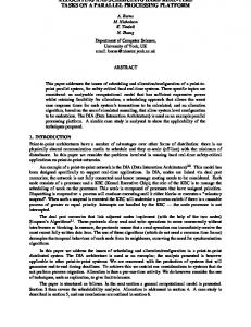
etc.) to build up proof plans that help the prover of the object level language to find the solution. The application of reflection techniques to KBS has been widely used in the recent past [13,21]. These techniques are used with different representation goals: implementation of non-monotonic reasoning patterns [18,19], declaration of inference methods [20], architecture description [5]. In general, reflection mechanisms can be understood, in this context, as a clear separation between domain and control knowledge. Few systems have clear semantics, among which we can find OMEGA [13] and BMS [18,19]. Due to the need in AI of dealing many times with uncertain and/or imprecise information, a number of models for representing uncertainty and imprecision have been largely studied within the AI community. In order to have such a possibility of explicitly representing uncertainty, our system provides at the object level a family of representation languages based on multiple-valued logics. These logics will be used in this paper to implement a design reasoning task, but the issue of modelling patterns of uncertain reasoning within the system is out of the scope of this paper. For a deeper insight in this topic, the reader is referred to [2,3]. Modularization is a standard technique to manage the complexity of highly interacting systems, such as KBSs. A module can be understood as a functional abstraction, by fixing both the set of components it needs as input and the type of results it can produce. The internal body of a module can then be hidden from the rest of the system, and the non-desired interactions avoided. This technique has been used in the context of functional programming, Standard ML [12], and Logic Programming [15]. In the architecture proposal of this paper, MILORD II, both techniques, reflection and modularization, are combined in order to be able to define complex reasoning patterns in the large. In Figure 1 you can see how a KB looks like in MILORD II. It consists of a set of hierarchically interconnected modules, each one containing an Object Level Theory (OLT) and a Meta-Level Theory (MLT) interacting through a reflective mechanism. Each module has also an import/export interface. The user of a KB provides information to modules via the import interface, and modules provide information to the user or to other modules via the export interface.

2

Import

Export OLT

Import

Export

MLT

Import

Export OLT

OLT •••

MLT

MLT Figure 1. Milord II KB structure.

The paper is structured as follows. In the second section the object level, based on multiple-valued logics, is presented and formalised. The next three sections are devoted to the meta-level language, the reification and reflection processes, and the dynamics of the execution of a module respectively. In Section 6 a declarative backtracking mechanism is presented, and in Section 7 a brief description of the MILORD II architecture is made. Finally, the example of the scheduling task proposed in the workshop as an instance of complex reasoning task is presented, followed by the traces of two test cases.

2. The Object level Reasoning at the object level in one module is generically based on the use of multiplevalued logics. A particular logic can be specified inside a module by defining which is the algebra of truth-values, i.e. which is the ordered set of truth-values and which is the set of operators associated to them. The kind of algebras of truth-values allowed in MILORD-II are those defined as follows: Definition An ordered Algebra of truth-values is a finite algebra A n,T = such that: 1) The ordered set of truth-values A n is a chain of n elements: 0 = a1 < a2 < ... < an = 1 where 0 and 1 are the booleans False and True respectively. 2) The negation operator Nn is an unary operation defined as Nn(ai) = an-i+1, the only one that fulfils the following properties:

3

N1: if a < b then Nn(a) > Nn(b), ∀a ∈ An, ∀b ∈ An N2: Nn2 = Id. 3) The conjunction operator T is any binary operation such that the following properties hold ∀a, b, c ∈ An: T1: T(a,b) = T(b,a) T2: T(a,T(b,c)) = T(T(a,b),c) T3: T(0,a) = 0 T4: T(1,a) = a T5: if a ≤ b then T(a,c) ≤ T(b,c) for all c 4) The implication operator IT is defined by residuation with respect to T, i.e. IT(a,b) = Max {c ∈ An | T(a,c) ≤ b} Such an implication operator satisfies the following properties: I1: IT(a,b) = 1 if, and only if, a ≤ b I2: IT(1, a) = a I3: IT(a, IT(b,c)) = IT(b, IT(a,c)) I4: if a ≤ b, then IT(a, c) ≥ IT(b,c) and IT(c,a) ≤ IT(c,b) I5: IT(T(a,b), c) = IT(a, IT(b,c)) As it is easy to notice from the above definition, any of such truth-value algebras is completely determined as soon as the set of truth-values and the conjunction operator T are determined. So, varying these two characteristics we can obtain a parametric family of different multiple-valued logics. In this way, each module can have a local type of reasoning, potentially different from others. Additionally, in order to allow a flux of information between modules and submodules with different local logics, renaming mappings between sets of truth values can also be specified inside a MILORD II module. In the same way as in classical logic we distinguish syntactically A from ¬A (A being a formula) because the only two truth value assignments to A are true or false in our case we need a syntactical representation for each truth value assignment to a formula A. This is necessary to allow explicit reasoning with the whole set of truth-values, i.e. to allow the presence of truth-values in the definition of the inference rules. On the other hand, even in the many-valued setting, partiality in the available information may lead to deal with imprecision at the truth level [7], i.e. one may know that a proposition must take a truth-value but doesn't know exactly which, and then no single value but a set of possible values (where the truth-value belongs for sure) is given instead. Moreover, having precise information does not always assure (see Section 2.2) to keep precision through inference processes, namely in Modus Ponens. This kind of imprecision can be handled by attaching intervals of truth values to formulas: the more imprecision there is, the larger the intervals are. In such a calculus the set inclusion relationship accounts for an imprecision ordering in the set of intervals of truth values. Namely, if [a,b] ⊆ [c,d] we say that [c,d] is at least as imprecise as [a,b], where a, b, c, and d belong to A n . Then, the language we propose in Section 2.1 is such that sentences are pairs of type (p, V) where p is a classical-like sentence and V is an interval of truth values, possibly empty (represented as []). Moreover, this representation leads to single satisfaction and entailment relations (see Section 2.2), rather than having classical sentences but several satisfaction and

4

entailment relations, as for example in [18]. Another related approach, based on modal operators instead of truth intervals, is the 3-valued non-monotonic logic NML3 [8]. It is worth noticing that, for instance, partial logics based on Kleene's or Belnap's multiple-valued logics can be modelled inside this framework. Belnap's 4-valued logic corresponds to the Algebra of truth-values with A 2 = {0, 1}. Belnap's overdefined value is represented as the empty interval [], and Belnap's undefined value is represented as the interval [0, 1]. Another interesting characteristic of the object level reasoning system is that deduction is based on what we call the "Specialisation Inference Rule" (SIR), a more general inference rule than Modus Ponens. Such a specialisation calculus is introduced in [14] to improve the input/output communication behaviour of the system . In the following description of the language, the semantics and the deduction system of a particular object level logic, we suppose an algebra of truth values An,T = fixed. 2.1. Syntax For the sake of simplicity, the syntax used in this Object Level Language description is a simplification of the actual MILORD II syntax (see Section 7). The propositional language OLn = (An, ∑O, C, OSn) of the object level is defined by: • A Signature ∑O, composed of a set of atomic symbols plus true and false. • A set of Connectives C = {¬, ∧, →} • A set of Sentences OSn whose elements are pairs of classical-like propositional sentences and intervals of truth-values. The classical-like propositional sentences are built from a set of atomic symbols and the above set of connectives, but restricted to literals and rules. That is, the sentences of the language are only of the following types: Literals: OLL = { (p,V) } Rules: OLR = {(p1 ∧ p2 ∧ ... ∧ pn → q,V*)1 } where p, p1, p2, ..., pn and q are literals (atoms or negations of atoms) with p i ≠ pj, pi ≠ ¬pj, q ≠ pj ∀i,j, and V and V* are intervals of truth-values. Intervals V * for rules are constrained to the upper intervals, i.e. of the form [a,1], where a > 0. Note: in the sequel we will identify intervals [a, a] with the value a.

2.2. Semantics The semantics is basically determined by the connective operators of the truth-value algebra An,T . Having truth-values in the sentences enables us to define a classical satisfaction relation in spite of the models being multiple-valued assignments. • Models Mρ are defined by valuations ρ, i.e. mappings from the first components of sentences to An such that: 1 The corresponding rule in MILORD II syntax would be:

If p1 and p2 and ... and pn then conclude q is V*

5

ρ(true )=1 ρ(false) = 0 ρ(¬p) = Nn (ρ(p)) ρ(p1 ∧ p2) = T(ρ(p1),ρ(p2)) ρ(p → q) = IT (ρ(p),ρ(q)) • The Satisfaction Relation between models and sentences is defined by: Mρ •O (p, V) iff ρ(p) ∈ V It is easy to see that the corresponding semantical consequence relationship between sets of sentences and sentences satisfies the following properties: SR1: (p,V) •O (¬p,W) ⇔ N*n(V) ⊆ W SR2: {(p,V1),(p,V2)} •O (p,W) ⇔ V1 ∩ V2 ⊆ W SR3: {(pi,Vi),(p1 ∧ ... ∧ pn → q,V)} •O (p1 ∧ ... ∧ pi-1 ∧ pi+1 ∧ ... ∧ pn → q,W) ⇔ MP*T(Vi,V) ⊆ W, where N*n and MP*T are the point-wise extensions1 of Nn and MPT respectively. MPT is a binary function from An to the set I(An) of intervals of An defined as:

 [] MPT(a,b) =  [a,1] T(a,b)

if a and b are inconsistent if b = 1 otherwise

where a and b are inconsistent if there exists no c such that I(a,c) = b MP T (a, b) provides the set of all solutions in An for ρ(q) in the following equation system: ρ(p) = a ρ(p → q) = b which corresponds to a multiple-valued version of the classical Modus Ponens inference rule. Property I5 of implication connectives makes useful this function in SR3.

{

2.3. Deduction system The object level deduction system is based on the following axiom schemes: (AS-1) (¬¬p → p, 1) (AS-2) (p, [0, 1])2 on the following axioms (A-1) (true, 1) (A-2) (false, 0)

1 Actually, MP* is defined to give the minimal interval containing the point-wise T

extension. 2 In any case any proposition has a truth-value between 0 and 1.

6

and on the following inference rules: (RI-1) weakening: (p,V1) ¶O (p,V2) where V1 ⊆ V2 (RI-2) not-introduction: (p,V) ¶O (¬p, N*n(V)) (RI-3) composition: (p,V1), (p,V2) ¶O (p,V1 ∩ V2) (RI-4) SIR1: (pi,Vi),(p1 ∧ p2 ∧ ... ∧ pi-1 ∧ pi ∧ pi+1 ∧ ... ∧ pn → q,Vr) ¶O (p1 ∧ p2 ∧ ... ∧ pi-1 ∧ pi+1 ∧ ... ∧ pn → q, MP*T(Vi,Vr)) From properties SR1, SR2 and SR3 of the semantical entailment, it is easy to check that this deductive system is sound. Theorem 1 (Soundness). Let A be a sentence and Γ a set of sentences. Then, Γ ¶O A implies Γ •O A. On the other hand, it is also straightforward to check that our deductive system is not complete. For instance, we have {(p → q, 1), (q → r, 1)} •O (p → r, 1), but {(p → q, 1), (q → r, 1)} ‡O (p → r, 1). However we can show that the system is complete for literal deduction, i.e., any literal that is semantically entailed by a set of formulas is also deducible from that set of formulas, generalising the literal completeness theorem of [19]. Theorem 2 (Literal Completeness). Let Γ be a set of formulas, (p, V) a literal. Then Γ •O (p,V) implies Γ ¶O (p,V) The proof of these theorems can be found in the long version of [14]

3. The Meta-level The meta-level language is a classical first order language ML = (∑M, C, MS) defined by: • A Signature ∑M = (Σrel, Σfun, Σcon, Σvar), where Σ rel = A set of atomic predicate identifiers plus Ass, Res, K, WK and P (with special semantics, see Sections 4-6). Σfun = A set of classical arithmetic function symbols. Σcon = A set of constants including the truth values and names for object propositional symbols. Σvar = A set of variable symbols; it can be empty. • The same set of connectives C as in the object language. • A set of sentences MS = MLLG ∪ MR where: 1 A discussion and motivation of this inference rule can be found in [14].

7

1.- MLLG is the set of ground literals, in a classical sense, from ∑M. 2.- MLR is the set {p1 ∧ p2 ∧ ... ∧ pn → c | pi and c are literals from ∑M } of metarules, where every variable occurring in c must occur also in some p i. Variables in meta-rules, if any, are considered universaly quantified. The semantics of the language is a first order classical one. The meaning of the special predicates K, WK and P will be explained when defining the reification function (Section 5), which gives sense to these predicates as a representation of object level sentences, and the meaning of Ass and Res will be explained when talking about the declarative backtracking mechanism (Section 6). The deduction system is based on only one inference rule: p1 ∧ p2 ∧ ... ∧ pn → c, p1', p2', ..., pn' ¶M c' where p1'... pn' are ground instances of p1 ... pn respectively, such that there exists a unifier σ for {p1 ∧ p2 ∧ ... ∧ pn , p1' ∧ p2' ∧ ... ∧ pn' }, and c'= cσ is the ground instance of c resulting from σ.

4. Dynamics of the reasoning process A complex KB consists of a hierarchy of modules. Each module contains an Object Level Theory (OLT) and a Meta-Level Theory (MLT). A module computes values for the propositions contained in its export interface; i.e. it computes the truth intervals for such propositions. A module execution consists of the reasoning process necessary to compute the values for some of the propositions in the export interface, those the user is interested in (the user can actually select a subset of the export interface when he orders the execution of a module). The execution of a module can activate the execution of submodules in the hierarchy. These executions only interact with the parent module through the export interface of the submodules, giving formulas back as a result. So, submodule execution extends the OLTs of modules by adding to them the formulas returned. It is worth noticing that the interaction is made only at the object level (see Figure 1). The reasoning process will be described in terms of variations of the Object Level Theories1 and Meta-Level Theories. The initial OLT of a module consists of its set of rules, i. e. a partial KB. The same holds for the MLT, which initially consists of the set of meta-rules. Definitions 1 Theories are considered not closed under deduction. So, they are closer to the concept

of presentation.

8

• We call an object-level elementary extension the extension of the OLT by a single literal. This can be done either by inference on the OLT, or by importing a piece of data either from the user (as specified in the import interface), from a submodule OLT or from the current MLT. • We call a meta-level elementary extension the extension of the current MLT by the set of ground literals resulting from the application of a single meta-rule over all the possible instantiations of its premise. The communication between OLTs and MLTs is done through reification and reflection processes that are explained in detail in the next section. Here, and as a rough introduction, we can say that a reification process maps sentences of the object level into sentences of the meta-level, whereas a reflection process maps meta-level sentences into object-level sentences, verifying reify(reflect(A)) = A. The reasoning dynamics follows the next schema.

STEP 1: The user selects a module to begin the system execution. The current OLT is the set of rules of the module, the current MLT is the set of meta-rules plus the instances of the user defined meta-predicates. These instances are given when defining the dictionary of a module (see Section 7). STEP 2: The reasoning process starts at the object level with the current OLT. If no elementary extension of the OLT is produced then STOP, otherwise, after the extension has been obtained the reasoning process control is passed to the meta-level (STEP 3). STEP 3: When the meta-level gets the control it builds the current MLT as the previous MLT plus the axioms coming from the reification of the current OLT. Then the meta-level reasoning process is activated. If no extension of the MLT can be obtained, the control is passed back to the object-level without extending the current OLT, i.e. the reflection does not modify the current OLT. On the other hand when an inference can be performed, and thus a meta-level elementary extension is made, the control is passed to the object level extending the current OLT by adding the reflection of the computed extension of the MLT1 . In any case the control goes to STEP 2. This dynamic process goes on till no possible extension of the OLT can be made. Special mention has to be made about the two meta-predicates Ass and Res. These are used to implement hypothetical reasoning patterns as will be described in Section 6. 1 So, in fact, the object-level will pass immediately the control to the meta-level. The

implementation has to take care of the unnecessary passing to and back of the control. This is the implicit iteration construct provided in MILORD II.

9

5. Reification and reflection The reification correspondence relates a subtheory of the OLT with the set of ground literals of the meta-language MLLG. Definition. We define the minimal literal OLT as OLTl* = { (p, W) | p literal and W = {Vi | (p, Vi) ∈ OLT}}

∩

A small set of meta-predicates is necessary to relate the OLLs with MLLG. For each one the corresponding reflection rules are defined. Given that the constant names used in the MLT are exactly the same as those used in the OLT as proposition names, the renaming operation, d e, is omitted,

5.1 Meta-predicate K K(p, V) means that V is the minimal interval such that the proposition (p, V) belongs to the OLT. There is a closed world assumption on this predicate. The upward reflection rules are: (p, V) OLT l* ¶M K(p,V) (p, V) ‹ OLTl* ¶M ¬K(p,V) The downward reflection process maps the meta level K predicate instances into object level literals. Only instances of the K predicate are considered because the other related metapredicate Ass is transformed into several instances of the K predicate in different MLT extensions, see Section 6. The downward reflection rule that relates MLT with OLT is defined as: ¶M Κ(p, V) ¶O (p, V)

5.2 Meta-predicate WK WK(p,V) means that (p, V) is deducible in the OLT, i.e. OLT ¶O (p, V). ¬WK(p, V) means that OLT ¶O (p, V') with V' ≠ [0, 1] but V' ¤ V (p, V) ∈ OLTl* and V ™ V* ¶M WK(p,V*)

10

(p, V) ∈ OLTl* and V ¤ V* ¶M ¬WK(p,V*)

5.3 Meta-predicate P P(p) means that (p, V) belongs to the deductive closure of OLT being V ≠ [0, 1]. If at the moment of the reification the computing of the deductive closure for p is not finished neither P(p) nor ¬P(p) will be generated. OLT ¶O (p, V) and V ≠ [0, 1] ¶ M P(p) OLT ‡O (p, V) and V ≠ [0, 1] ¶M ¬P(p)

With these reflection rules we can differentiate between different sorts of partiality in the information: • propositions that have not yet been the goal of the prover, {p| ∀ V≠[0, 1], ¬K(p, V) }, • propositions provisionaly unknown, {p| K(p, [0, 1]) }, and • propositions that are definitively unknown because they cannot be proven {p| ¬P(p) }.

6. Declarative Backtracking There is a main difference between reflecting an instance of the predicate K and an instance of the predicate Ass. When we reflect K(p, V) all future extensions of OLT will contain the fact (p,V), whereas when we reflect Ass(((p1 , V1 ), (p2 , V2 ))), any future extension of OLT will contain at least one of the elements of the argument set of Ass, i.e. (p1, V1) or (P2, V2). More concretely, when a meta-rule with an Ass predicate in its conclusion is applied, as many extensions of the meta-theory MLT as elements in the argument set of the Ass predicate are generated. For instance, consider the case where, in a certain moment, we have in the current object theory only the literal (p, 1) and MLT consists of the following meta rule: M0001 If K(p, 1) and ¬P(q) then Ass(((q, 1), (q, 0)))

11

Suppose also that q could not be proved in OLT. Then, after the reification process, the current MLT will be the extension of the previous one with the ground literals K(p, true) and ¬P(q). So, now the above meta-rule can be applied, and this causes the system to obtain the conclusion Ass(((q, 1), (q, 0))). The meaning of the meta-predicate Ass is that the elements of its argument should be assumed in different extensions of the current OLT. This is done by building a tree of MLTs, each containing a K metapredicate instance for all the elements of the argument of Ass. So in this case we obtain the following two different extensions of the current MLT: MLT1 = MLT ∪ K(q, 1) MLT2 = MLT ∪ K(q, 0) MLT K(p, 1) ¬ P(q) ASS MLT1

K(p, 1) ¬ P(q) K(q,1)

K(p, 1) ¬ P(q) K(q, 0)

MLT2

Figure 2. Meta-theories branching using the Ass meta-predicate. From now on, and until another instance of an Ass predicate or a Res predicate is obtained, the existing communication (reification and reflection) between OLT and MLT is moved to a communication between OLT and MLT1 . Thus, in this case, after the reflection process OLT is extended with (q, 1). In order to backtrack in the tree of MLTs generated by successive applications of Ass predicates, the system provides a special 0-ary predicate Res. When a meta-rule concluding Res is applied, we perform a backtracking in the meta-theories tree. This backtracking restores the parent MLT, and consequently the current OLT becomes the OLT which was active at the moment the assumptions were made by the parent MLT. In the above example, backtracking from MLT1 to MLT makes that q will not be true in the current OLT, and that immediately the communication (reification and reflection) between OLT and MLT is moved to a communication between OLT and MLT2 (see next figure).

12

MLT K(p, 1) ¬ P(q) Res MLT1

K(p, 1) ¬ P(q) K(q,1)

K(p, 1) ¬ P(q) K(q, 0)

MLT2

Figure 3. Backtracking using the meta-predicate Res. It is worth noticing that predicates Ass and Res provide the system with a declarative backtracking mechanism, similar to the approach taken in MetaProlog [4]. This declarative mechanism allows us to implement several complex reasoning patterns. For instance, consider that an assumption was made at the meta-level. Whenever a contradiction occurs in OLT afterwards, we can declaratively detect it, and then, by means of the Res predicate, we can move back to a previous non contradictory OLT. This can be achieved by a meta-rule, such as If Ass($y) and K($x, ()1) then Res

Ass can be used as a condition to check if an assumption has been previously made. Meta-level theories keep track of them to allow explicit reasoning about the assumptions active at any moment. Notice that a contradiction in OLT occurs when OLT contains literals of the form (p, V) and (¬p, V') such that V ∩ N(V') = Ø, and then the RI-2 and RI-3 inference rules are applied to generate (p, []). It is worth noticing that, in MILORD II, when at the object level deductions may be derived from a reflected fact, (p, V), it is better to use the Ass(((p, V))) predicate in the conclusion of meta-rules because afterwards and using a Res meta-predicate we will be able to recover the present state if something goes wrong. Conclusions made by a meta-predicate K are irrevocable. We can see the Ass meta-predicate as a pointer (copy of the state) we put in our reasoning process in order to retract what is deduced from it later on, if necessary.

7. MILORD II Language description MILORD II is a currently working expert systems shell which contains the features described up to now, and others that are out of the scope of this paper. The interested reader is referred to [1,2,16]. We will concentrate on the description of the modular structure of the language, necessary to understand the next sections of the paper. 1 In MILORD II intervals are represented between parenthesis instead of brackets.

13

The language provides three basic mechanisms of module manipulation: 1) Composition of modules through the declaration of submodules, 2) Refinement of modules, and 3) Composition of modules through operators defined by the user via generic modules definition. Next, a description of the different components of a MILORD II module is made. Then, generic modules are presented. Afterwards two basic operations on modules are outlined: Combination and Refinement. Combination is used to build up the hierarchical structure of modules. Refinement is used, in what matters here, to perform inheritance between modules. Given the space at hand the MILORD II description will necessarily be just a glimpse. 7.1. Modules The basic KB units of MILORD II are modules. Modules are compound structures. The basic elements that compose a module are: • Import interface: information to be provided by the user 1. • Export interface: output result of a module. • Object level knowledge: an initial Object Level Theory. • Meta-level knowledge: an initial Meta-Level Theory. Next a detailed description of the basic components of a module and some syntax elements are presented.

Import interface Imported facts2 are those whose values are fixed at run time by the user. The import interface is defined by an expression like: Import fact1, fact2,..., factn

No other facts inside the module will receive values from the user. In other words, this set of facts is the only way in which a user can influence the results of a module.

Export interface Exported facts are those that are visible from outside the module; visible either by users or by other modules. The values of exported facts can be fixed by the OLT, by the MLT

1 Modules can also import information from other modules via their declaration as

submodules. See Section 7.3. 2 The MILORD II object level contains not only multiple-valued propositions, but also numerical variables, variables defined by enumeration and boolean propositions. As a general term we use fact to refer to any of them. A very informal definition of fact might be: an object level representation unit that can receive a value, whatever it is, by the user or by the system.

14

or by the user if an exported fact is also an imported one. The export interface is defined by an expression like: Export fact1, fact2, ..., factm

Facts not mentioned in the export interface are hidden to the user and to the rest of the modules (i.e. their values cannot be consulted). The export interface is the only mandatory component of a module. A module with no exported facts is meaningless.

Object level knowledge The object level of a module is composed of: a) Dictionary : this component defines the fact identifiers and some attributes of them, for example their type, and the way their values are computed. The value of a fact is obtained either by a question to the user (Question attribute), by a LISP function computation (Function attribute) or by deduction if none of the previous atributes appear in the fact definition. It also defines relations between facts, i.e. meta-predicate instances. For example:

Dictionary: Predicates: ... Temperature =

Corporal-surface =

Name: "Patient's Temperature (in centigrade)" Question: "Which is the patient's Temperature?" Type: Numeric Relation: less-relevant-than AIDS Name: "Patient's Corporal Surface (in m2)" Type: Numeric Function: (* 0.024265 (expt heigth-in-cm 0.3964) (expt weigth-in-kg 0.5378))

... ;; within the Temperature predicate definition the next meta-predicate instance is present: ;; less-relevant-than(Temperature, AIDS) ;; heigth-in-cm and weight-in-kg are numerical facts, belonging to the same ;; dictionary definition but not defined in this example.

b) Rules: the set of rules of the object level. For example: R0005 if fever > 38.5 and shivers then conclude bacterian-disease is sure1

It is possible to use two special propositions true and false as conditions. These propositions always evaluate to the maximum and minimum certainty values of the multiple-valued logic used in the module respectively. So, it is possible to write rules as:

1 Given that rules always have intervals of the type [a, 1] these intervals are written in

MILORD II as just a.

15

if true then conclude p is moderately-possible

c) Local logic: it is possible to define three main components of an Inference System.: (i) the set of truth-values, (ii) a renaming mapping between the truth-values of the submodules, if any, and the truth-values of the module that combines them and (iii) the connective operators used to combine and propagate the truth-values when making inference. A more complete description can be found in [3].

The next piece of code is an example of module definition containing rule and logic declarations. Module Previous_Treatment = Begin Import Prev_Treat Export Penicillin, Tetracycline Deductive knowledge Dictionary: not defined here Rules: R001 If Prev_Treat = (Peni) then conclude Penicillin is sure R002 If Prev_Treat = (Peni) then conclude Tetracycline is impossible Inference system: Truth values = (impossible, sure) Connectives1: Conjunction: ( (impossible, impossible) (impossible, sure)) Disjunction: ( (impossible, sure) (sure, sure)) end deductive end

Meta-level knowledge The current implementation of the meta-language allows the definition of meta-rules (as explained in previous sections), and the type of module execution, which can be lazy or eager. Lazy means that facts are evaluated, at the object level, only when needed, i.e. imported facts and exported facts of submodules are asked only if they may be useful to compute the export interface of the module. On the contrary an eager module execution obtains, first of all, values for the imported facts and for the exported facts of the submodules and then the deductive knowledge is used. The interaction between OLT and MLT (reification/reflection step) is made after every import information is obtained, after every submodule execution and after every time OLT is extended by deduction.

1 Connectives may be defined, as in this case, as a truth-table, represented by rows, and

following the order of the linguistic terms. In the conjuntion definition of this example module it is represented that: impossible ∧ impossible = impossible, impossible ∧ sure = impossible, sure ∧ impossible = impossible, sure ∧ sure = sure, that is, the classical boolean and connective.

16

The next example is taken from the application on scheduling explained in Section 8. In it you can observe the diverse components explained above. Module Requirements1 = Begin Export A1, A2, A3, A4 Deductive knowledge Dictionary: predicates: A1 = Name: "A1" Type: logic A2 = Name: "A2" Type: logic relation: diff A4 A3 = Name: "A3" Type: logic relation: before A2 relation: before A4 A4 = Name: "A4" Type: logic Inference system: Truth values = (false, t1, t2, t3, true) end deductive control knowledge evaluation type: eager end control end

7.2 Generic Modules Generic modules are the way to define functions from modules to modules. They work in a way similar to a linker in a programming language. An example of a Generic Module is the next one: Module G(X : S1; Y : S2) : S3 = Begin ;;Usual module definition. ... End

This generic module accepts two modules as parameters satisfying the refinement relation with S1 and S2 respectively, and produces a module satisfying the refinement relation with S3 (see Section 7.4). These generic modules can be defined at top level or at any level in the hierarchy of modules. In this sense it differs from the treatment of Functors in Standard ML [12]. In the generic module referring to parameters X and Y is allowed. The compiler is responsible of applying the generic modules to their actual parameters, i.e. generic modules are static, they cannot be applied at run time. 7.3. Combination of modules We say that a module combines other modules when it has access to their exported facts. It can be done in two ways: (1) declaring submodules, and (2) applying a generic module. The declaration of submodules is identical, syntactically, to the declaration of modules, and is the key to the hierarchical organisation of KBs. The distinction between a KB and a piece of a KB is lost in MILORD II, and a KB will be then a module, may be containing other modules as submodules.

17

A generic module can be seen as a module with some submodule names, the name of the arguments, not linked to any particular module. At the moment of the application those submodule names are linked to the particular modules given as parameters (see next figure).

Module G(X: S1; Y: S2) : S3 = Begin ... End

Module A = G(B, C) GENERATES

Module A : S3 = Begin Module X : S1 = B Module Y : S2 = C ... End

Figure 4. Generic Module application. In both cases, i.e. a module which combines its submodules or a generic module applied over some parameters, the resulting module may use, in its rules and meta-rules, the facts appearing in the export interfaces of the modules declared as submodules and/or the parameters. The access to the exported facts is made using a prefix mechanism. An exported fact is identified by two components: 1) a path of module names, separated by "/", indicating how to access to the fact in the hierarchy of modules, and 2) the name of the fact, i.e. name1 / name 2 / ... / namen / fact_name These combinations of modules build up a hierarchical structure of modules. Each module containing their particular object level and meta-level theories.

7.4. Inheritance through module refinement Module refinement is a mechanism that allows to incrementaly construct knowledge bases. The refinement operation takes two modules and gives another module as result. The resulting module is essentially equal to the first argument but contains elements of the second argument not defined in the first, i.e. implements a kind of inheritance. Elements that are inherited are dictionary entries and local logics. That is, if the second argument contains a dictionary entry that is not present in the first one, it is inherited. Similarly, if the first argument does not have a local logic definition it is inherited from the second. The refinement operation is also used to verify if the first argument is an enrichment of the second and to make information hiding [17]. To express that a module C is the result of the refinement between A and B we write Module C = A : B

or Module C : B = A

18

both expressions are equivalent. 7.5 Environment and working procedure The MILORD II system consists of two main components: (1) a compiler that checks the code of the KB to detect errors, to solve dependencies in the declaration of submodules, to compute the modules resulting from the application of generics, and (2) an interpreter that executes the code generated by the compiler. Code

KB

Interpreter

Compiler

User Errors Figure 5. MILORD II KB execution procedure. The user, when running a KB selects a module and then the interpreter executes it, The interpreter will compute the value for the export predicates of that module and will give them back to the user. In the execution process the user will be asked for the information necessary to compute the results.

8. Specification of the scheduling reasoning system 8.1. Design reasoning systems In general, to specify a complex reasoning system it is necessary to define a hierarchy of modules. This hierarchy captures the task/subtask decomposition. This is clear in diagnosis reasoning systems (see for example, PNEUMON-IA [22]). However, in a design reasoning system (DRS) the possibility to iterate over a set of subtasks (hypothesis assumption, evaluation, and revision) plays a fundamental role. The only way to perform iteration in our language is through the reification/reflection mechanism. This leads to understand the task/subtask decomposition as a particular relation between the OLTs and the MLTs. To specify a DRS we build a module in which we associate to each design variable a proposition identifier. The space of values for variables is understood in the proposed

19

implementation as the set of truth values of a particular multiple-valued logic 1 . Requirements are expressed as restrictions over the truth value assignments for these propositions. Solutions to the design process are then considered to be truth value assignments that fulfil the requirements. In order to find a solution, the module representing the design task is executed till a final OLTl* is found. This is done through the interaction of the OLT and MLT of the module. The MLT extends the OLT by reducing the set of possible truth values for the propositions (possible models), initially the whole interval [0, 1] of truth values. This reduction is done using heuristics that allow to prune part of the search space. The final OLT l* will consist of a set of literals (p, V) where p is a proposition representing a design variable and V an interval of truth values. These intervals represent all the non rejected possible values for those variables. When the execution finishes, the truth value assignment ρ representing a correct solution can be built up from the literals (p, [v 1, v2]) belonging to the final OLTl* making ρ(p) = v1.. In the sequel the modular structure and the different subtask specifications of the DRS in a scheduling framework, as described in the workshop proposal, are described. 8.2. Modular structure of the scheduling reasoning system (SRS) In order to implement a scheduling task with a set of requirements to be fulfilled, two modules must be defined: • Requirements module This module will contain the requirements as meta-predicates over the propositions of the object level, i.e. restrictions over the possible values that object level propositions can take. These meta-predicates are defined in the dictionary of the module. This module also defines the particular multiple-valued logic for the object level. However, in the example task there is no truth-values combination, so selecting connectives is irrelevant. • Design task Module This module contains the initial conditions of the problem as object level rules, and the meta-rules that perform the different subtasks of the scheduling process. Each problem setting (number of tasks and relations between them) requires a particular requirements module and a particular design task module. All design task modules have the MLT in common. Thus, to build the actual module that will perform the design, it is necessary to connect the particular design task module with the requirements module, so the former can inherit the requirements of the problem from the later. It is done in the following way, using the refinement operation:

1 This is the approach followed in this paper. Given that the MILORD II object

language is a bit richer than the object language presented here, we could have done it using numerical variables for example.

20

Module example = design : requirements1

8.3. Subtask specification of the SRS The subtask decomposition of the scheduling problem is embedded into the design module components. Next the different subtasks and their relation with meta-level constructs will be described. 8.3.1. Requirements Generation This task is performed by the user through the definition of the requirements module, explained in the previous section, with the particular set of requirements to be fulfilled by the scheduling solutions. The requirements of the scheduler under study are: - The number of tasks to be scheduled, - The temporal relations between them, and - The number of available time points. The tasks will be defined as a set of object level propositions A1, ..., An, the temporal relations as meta-predicates over pairs of elements in the set {A 1 , ..., An }, and the number of time points time1, ..., timeq as the truth-values of the logic, which will be (0, time1, ..., timeq, 1). In our particular case there are four types of requirements that we will represent by four meta-predicates: before, equ, diff and notbefore. 1.- before(x, y) means that activity x must occur before activity y. 2.- equ(x, y) means that activities x and y must occur in the same time period. 3.- diff(x, y) means that activities x and y must not occur in the same period. 4.- notbefore(x, y) means that activity x must not occur before activity y. Meta-predicates are defined (see Section 7.1) in the dictionary within the definition of the propositions, i.e. the tasks. Therefore, a schema of the requirements module definition would be: Module Requirements = Begin Export A1, ..., An Deductive knowledge Dictionary: predicates: ... Ai = Name: "Taski" Type: logic

relation: reli,j Aj ... relation: reli,j+m Aj+m

... Inference system: Truth values = (false, time1, ..., timeq, true) end deductive control knowledge evaluation type: eager end control

1 Remember that A:B is a modular expression that generates a new module that results

from modifying A by adding elements inherited from B, such as dictionary or logic.

21

end

Where relk,l stands for an element of {before, equ, diff, notbefore}. 8.3.2. The scheduling search space The description of the KB that specifies the scheduling task will be done in terms of its associated search space. In this search space the nodes represent the set of possible solutions, that is, all the possible assignments we can build from the proposition truth intervals. Each child represents a subset of the possible solutions of the parent node obtained by reducing the truth-interval of one proposition. There are two ways of doing that: increasing the lower bound or decreasing the upper bound of the truth-interval. The former corresponds to an "as soon as possible" assignment heuristic and the latter to an "as late as possible" assignment heuristic1. Depending on the heuristic associated to each meta-predicate we can select for each node the best possible assignment. Once an assignment is chosen for a node, it is evaluated. If no requirement is violated, that assignment is a solution. Otherwise, i.e. if some requirement violations are detected, one of them is heuristically selected to be solved. Then the solution of the selected requirement violation is done by pruning all the child except those that contain no assignment violating that requirement. It is easy to see that all the remaining possible solutions are those contained in the non cut children. If there remains more than one children a search with backtracking has to be performed. Backtracking is done when we are at a leave node and the single solution it represents is found to violate a requirement. In the example considered this general schema is particularised by: • The assignment heuristic is "as soon as possible" for all propositions. So, the best assignment for each node is the one with the lowest truth values. • There are four types of requirements: before, equ, diff and notbefore. The requirement violation of three of them, before, equ, and notbefore, makes that the pruning process leaves only one children, whereas the diff violation leaves two. There are two possible solutions of a diff violation: increase the lower bound of the interval of one of the two conflicting tasks. So, trying to gain efficiency, the implemented heuristics is to solve any of the former before solving the latter, because in that way branching is generated as late as possible. 8.3.3. Implementation of the heuristic search The implementation of the heuristic search is done by defining a set of rules and metarules. Rules are responsible for the initial attachment of the whole space of values to the propositions and meta-rules are responsible for the pruning of the search space. For each proposition Ai representing a scheduling activity a rule like R000i if true then conclude Ai is time1

has to be written in order to define the initial possible truth-values for the propositions, i. e. the interval [time1, true]. These intervals represent the root node of the search space. 1 In our system these heuristics could be specified for each meta-predicate.

22

In general the truth-value of the rules determine the initial time point to start the scheduling of the corresponding activity. So initial conditions of the problem can be stated just modifying the certainty values of these rules. At the meta-level, for each possible requirement violation a meta-rule is written, having as premise a set of conditions that are true when a particular requirement violation is produced, and as conclusion "how" to restrict the set of possible values for one activity in such a way that the violation is solved. That is, the meta-rule cuts off a set of children states. Meta-rules can be of two types depending on the requirement violation: A.- Meta-rules that restrict the possible values of propositions in such a way that there is no need for backtracking, i.e. only one child remains. This is the case of requirements of type before, equ and notbefore. These meta-rules use the K meta-predicate in their conclusion. An example of such a meta-rule for the before requirement is: M002 if before($x,$y) and K($x,($z true)) and K($y, ($w true)) and ge($z,$w) then conclude K($y, (suc($z) true))

B.- Meta-rules that perform branching, i.e. two children remain. This is the case of requirement diff. These meta-rules have the meta-predicate Ass in their conclusion. Example: M005 if diff($x,$y) and K($x,($z true)) and K($y,($z true)) then conclude Ass((($x,(suc($z) true),($y,(suc($z) true))))

A special meta-rule is also needed to detect when no solution is found, and then in that case to backtrack. This situation can be detected when a proposition gets the interval [1,1] as follows: M001 if K($x, (1 1)) and type($x, logic) then conclude Res

When the search space is exhausted and no solution is found, this situation reflects that the set of requirements is inconsistent. 8.3.4. Relationship between the implementation and the subtask decomposition of the scheduling problem In the workshop proposal of the Example Reasoning Task Description [***] a subtask decomposition of the scheduling problem is suggested. It is possible to identify these subtasks in our implementation. 1. Requirements generation. This is a particular module defined by the user, as described in a previous section. 2. Assumption generation. Whenever a reflection is made, the truth-intervals assigned to propositions represent all possible assumptions for each of them.

23

3. Assumption selection. Whenever a reification is made, lower bounds of the truthintervals appearing in instances of predicates K represent the selected assumptions for all the propositions. 4. Design object evaluation. Whenever a premise of a meta-rule becomes true, a particular requirement violation is detected. In this case, the solution represented by the current assumptions is not correct. If no premise becomes true, every requirement is fulfilled, and thus the current assumptions are a solution. Given that in this implementation propositions always have an assigned value, the existence of a requirement violation is equivalent to the non-satisfaction of the requirement. 5. Design process evaluation. When a requirement violation is produced, the premise of some meta-rule becomes true, and is activated. Depending on whether there are still solutions to be tested, the possible actions the meta-rule can take are either retract univocaly the assumption of a particular proposition (using meta-predicate K), or branch over two possible retractions for different assumptions (using meta-predicate Ass). Otherwise, the meta-rule takes a backtracking action (using the meta-predicate Res). 6. Assumption revision. In the case of a meta-rule deducing an instance of predicate K, this subtask is coincident with Assumption Generation. In the case of an Ass predicate, one of the elements of the argument set is selected and considered to be as a K predicate instance, and then we are again in the case of an Assumption Generation. Finally, in the case of a Res predicate, the state in which the most recent Ass predicate has been deduced is recovered and thus, after the reflection is made, the propositions recover the values they had in that state. 8.4. Scheduling Code schema Next you can see the scheduler schema. This module code collects the different subtasks explained above.

Module Scheduler_n = Begin Export A1, A2, …, An Deductive knowledge Rules: R001 if true then conclude A1 is t1 R002 if true then conclude A2 is t1 … R00N if true then conclude An is t1 end deductive Control knowledge Evaluation type: eager

24

Deductive control1: M001 if K($x, (1 1)) and type($x, logic) then conclude res M002 if before($x,$y) and K($x,($z true)) and K($y, ($w true)) and ge($z,$w) then conclude K($y, (suc($z) true)) M003 if equ($x,$y) and K($x,($z true)) and K($y,($w true)) and gt($z,$w) then conclude K($y, ($z true)) M004 if notbefore($x, $y) and K($x,($z true)) and K($y,($w true)) and lt($z, $w) then conclude K($x, ($w true)) M005 if diff($x,$y) and K($x,($z true)) and K($y,($z true)) then conclude ass((($x,(suc($z) true),($y,(suc($z) true)))) end control end

9. Examples and tests 9.1. Code of the example Here we present the complete code of the scheduling module for a set on 4 tasks to be scheduled. The set of requirements is specific for each example test and they will be presented in the next sections. Module Scheduler_4 = Begin Export A1, A2, A3, A4 Deductive knowledge Dictionary Rules: R001 if true then conclude A1 is t1 R002 if true then conclude A2 is t1 R003 if true then conclude A3 is t1 R004 if true then conclude A4 is t1 end deductive Control knowledge Evaluation type: eager Deductive control: ;; If a fact gets the maximum value no solution can be found . M001 if K(=($x, $y) , (1 1)) and K(=(max-value, $y ), (1 1)) and type($x, logic) then conclude res M002 if before($x,$y) and K($x,($z true)) and K($y, ($w true)) ;; X before Y . and ge($z,$w) then conclude K($y, (suc($z) true)) M003 if equ($x,$y) and K($x,($z true)) and K($y,($w true)) ;; X equal Y and gt($z,$w) then conclude K($y, ($z true))

1 In the Meta-rules, it is possible to use some system-defined meta-predicates such as: ge

(greater or equal), lt (lower than), gt (greater than), type (type of reified fact). The metapredicates ge, lt, gt can be applied over the order of the truth-values of the local logic, or over the real numbers. It is also possible to perform operations on top of the truthvalues, such as suc (successor function), that have to be understood in the context of an ordered set of truth-values.

25

M004 if notbefore($x, $y) and K($x,($z true)) and K($y,($w true)) ;; X not before Y and lt($z, $w) then conclude K($x, ($w true)) M005 if diff($x,$y) and K($x,($z true)) and K($y,($z true)) ;; X different Y then conclude ass(($x,(suc($z) true),($y,(suc($z) true))) end control end

9.2. First Example To define the scheduler for the first test example we define a module requirements1 which contains the meta-predicates defining the relations between the propositions at the object level, and the set of truth-values representing the admissible time points. Module Requirements1 = Begin Export A1, A2, A3, A4 Deductive knowledge Dictionary: predicates: A1 = Name: "A1" Type: logic A2 = Name: "A2" Type: logic relation: diff A4 A3 = Name: "A3" Type: logic relation: before A2 relation: before A4 A4 = Name: "A4" Type: logic Inference system: Truth values = (false, t1, t2, t3, true) end deductive control knowledge evaluation type: eager end control end

Now, and using the inheritance property of the operator ":", we define the module that performs a scheduling of four tasks, module scheduler_test_1, with a particular set of requirements, defined in requirements1. Module Scheduler_test_1 = scheduler_4 : requirements1

Now, let's see the execution trace of the module Scheduler_test_1. Assumption generation: A1 (t1 true) A2 (t1 true) A3 (t1 true) A 4 (t1 true) Assumption selection: A1 t1 A2 t1 A3 t1 A4 t1 Design object evaluation: REQUIREMENTS VIOLATION Design process evaluation: K(A 2 , (t2 true)) K(A4 , (t2 true)) Assumption revision: A2 t2 A4 t2 Increasing the minimum value of the fact A2 from t1 to t2 Increasing the minimum value of the fact A4 from t1 to t2 Assumption Generation: A1 (t1 true) A2 (t2 true) A3 (t1 true) A4 (t2 true) Assumption selection: A1 t1 A2 t2 A3 t2 A4 t2 Design object evaluation: REQUIREMENTS VIOLATION

26

Design process evaluation: Ass(((A 2 (t3 true)) (A4 (t3 true)))) Assumption revision: A4 t3 Branching over MLTs: (#:G1112 #:G1113) Increasing the minimum value of the fact A4 from t2 to t3 Assumption Generation: A1 (t1 true) A2 (t2 true) A3 (t1 true) A4 (t3 true) Assumption selection: A1 t1 A2 t2 A3 t1 A4 t3 Design object evaluation: EVERY REQUIREMENT IS FULFILLED Design process evaluation: NIL Assumption revision: NIL ---FINAL ANSWER-----THE FACT A1 IS t1 THE FACT A2 IS t2 THE FACT A3 IS t1 THE FACT A4 IS t3 ---------------------------------9.3. Second Example Similarly to the previous test example we define the set of requirements with a module requirements2. Module Requirements2 = Begin Export A1, A2, A3, A4 Deductive knowledge Dictionary: predicates: A1 = Name: "A1" Type: logic relation: equ A3 A2 = Name: "A2" Type: logic relation: before A3 relation: diff A4 A3 = Name: "A3" Type: logic relation: equ A1 A4 = Name: "A4" Type: logic relation: before A3 Inference system: Truth values = (false, t1, t2, t3, true) end deductive control knowledge evaluation type: eager end control end

Finally the scheduler for this test example is built, Module Scheduler_test_2 = scheduler_4 : requirements2

Now, let's see the execution traceof Scheduler_test_2. Assumption generation: Assumption selection:

A1 (t1 true) A2 (t1 true) A3 (t1 true) A 4 (t1 true) A1 t1 A2 t1 A3 t1 A4 t1

27

Design object evaluation: REQUIREMENTS VIOLATION Design process evaluation: K(A 3 , (t2 true)) Assumption revision: A3 t2 Increasing the minimum value of the fact A3 from t1 to t2 Assumption generation: A1 (t1 true) A2 (t1 true) A3 (t2 true) A 4 (t1 true) Assumption selection: A1 t1 A2 t1 A3 t2 A4 t1 Design object evaluation: REQUIREMENTS VIOLATION Design process evaluation: K(A 1 , (t2 true)) Assumption revision: A1 t2 Increasing the minimum value of the fact A1 from t1 to t2 Assumption Generation: A1 (t2 true) A2 (t1 true) A3 (t2 true) A4 (t1 true) Assumption selection: A1 t2 A2 t1 A3 t2 A4 t1 Design object evaluation: REQUIREMENTS VIOLATION Design process evaluation: Ass(((A 2 (t2 true)), (A4 (t2 true)))) Assumption revision: A4 t2 Branching over MLTs: (#:G1089 #:G1090) Increasing the minimum value of the fact A4 from t1 to t2 Assumption generation: A1 (t2 true) A2 (t1 true) A3 (t2 true) A 4 (t2 true) Assumption selection: A1 t2 A2 t1 A3 t2 A4 t2 Design object evaluation: REQUIREMENTS VIOLATION Design process evaluation: K(A 3 , (t3 true)) Assumption revision: A3 t3 Increasing the minimum value of the fact A3 from t2 to t3 Assumption generation: A1 (t2 true) A2 (t1 true) A3 (t3 true) A 4 (t2 true) Assumption selection: A1 t2 A2 t1 A3 t3 A4 t2 Design object evaluation: REQUIREMENTS VIOLATION Design process evaluation: K(A 1 , (t3 true)) Assumption revision: A1 t3 Increasing the minimum value of the fact A1 from t2 to t3 Assumption Generation: A1 (t3 true) A2 (t1 true) A3 (t3 true) A4 (t2 true) Assumption selection: A1 t3 A2 t1 A3 t3 A4 t2 Design object evaluation: EVERY REQUIREMENT IS FULFILLED Design process evaluation: NIL Assumption revision: NIL ---FINAL ANSWER-----THE FACT A1 IS t3 THE FACT A2 IS t1 THE FACT A3 IS t3 THE FACT A4 IS t2 ----------------------------------

28

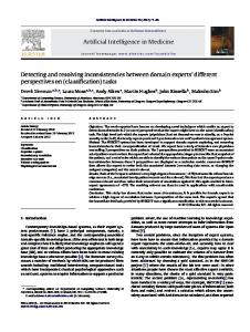
9.4 Summary of the executions In the next figure you can see the results obtained by the execution of the two sets of requirements proposed in this workshop.

A1 A2 A3 A4

A1 A2 A3 A4

t1 t2 t3 t1 t2 t3 Figure 6. Correct scheduling for the first example (left) and the second one (right). As a glimpse of the complexity of the proposed solution we can say that the complexity of the scheduling task is O (n 2 * m * p2 * 2q ) where n is the number of before relations, m is the number of equ relations p is the number of notbefore relarions and q is the number of diff relations. The complexity is considered as the number of proposition value modifications necessary to get a solution. In the two examples the number of reification/reflection steps is 2 and 5 for the first and the second examples, respectively. The heuristic of applying first the meta-rules that solve the before, equ and notbefore relations, seems to give an acceptable concrete complexity of the scheduler proposed. Further study seems, however, necessary.

10. Comparative study During the workshop a set of criteria was proposed in order to compare the different approaches. Below it is discussed to what extent these criteria are fulfilled by MILORD II. • Expressive Power MILORD II is provided with the expressive power of rule-based languages, augmented with the many-valued approach to uncertainty management at the object level language, and with modular constructs and operations. • Transparency, Clarity The language has a minimum number of different concepts, basically rules, meta-rules, propositions and meta-predicates. Also the combination of computational units to build up complex knowledge bases is simple and regular: declaration of submodules, refinement between modules and application of generic modules. • Knowledge Level

29

Although some of the characteristics of the Knowledge Level approaches, mainly the components of expertise [ref Steels], have been taking into consideration, there is no formal link between Knowledge Level concepts and MILORD II programming concepts. Nonetheless, some hints of this mapping could be: consider tasks as non-generic modules, methods as generic modules, and domain models as object level deductive components of modules. • Declarativeness Although there are some implicit mechanisms, such as the sequencing of rules or the reflection mechanisms, the MILORD II language is mostly declarative mainly because it is a rule-based language (both the object and meta-level languages) and therefore it shares the declarativeness of any logical language. • Specification of Dynamic Aspects In MILORD II it is possible to specify dynamic aspects of the reasoning process in a declarative manner at the meta-level of each module, by means of some special metapredicates. Among them, it is worth noticing that the Ass and Res predicates provide the system with a declarative backtracking mechanism. • Multi-level Specification The way to define multi-level specifications in MILORD II is through the refinement operation between modules. This operation allows to incrementally define the contents of a module, starting from a very general definition, containing just a module signature, up to a completely coded module. It is worthwhile to stress the fact that this refinement is not a single step operation, that is, the process to get the final content of module from a general starting specification can involve several applications of the refinement operation. • Specification of Reflective Reasoning Patterns One of the key capabilities of MILORD II is having the knowledge structured in each basic building block (or module) as an interacting pair composed of a theory and a metatheory. Such interaction is governed by upward and downward reflection rules that, together with the declarative backtracking mechanism, allows to specify different kinds of complex reasoning patterns. • Genericity MILORD II allows to define generic modules. Generic modules permit to reuse both the domain dependent knowledge and the control knowledge that are common to a set of modules. These modules will be used as parameters of the generic modules. As a matter of example, the specification of a generic problem solving method can be encoded as control knowledge in a generic module. • Specification of Integrated Systems Despite MILORD II has not yet specific functions to connect KBs to other programs, as explained in Section 7.1 it is possible to define LISP functions to compute fact values.

30

In this way there is a possibility through LISP to connect the system to other languages and applications. • Executability MILORD II is implemented in CommonLisp and is running on top of Macintosh computers. • Clear operational Semantics As explained along this paper, the object and meta level deduction and the reflection mechanisms are clearly understood from an operational point of view. The overall control algorithm is defined in these terms; see Sections 2 to 6. • Solid Formal Semantics The formal semantics of the object level language is defined in Section 2, and the semantics of the meta-language is defined in Section 3. However, a global formal semantics for the whole is still missing and is part of our future work. • Uncertainty MILORD II provides a family of representation languages based on the use of manyvalued logics at the object level. Truth values are a finite ordered scale of certainty weights with which the object level knowledge can be qualified. Both the set of truth values and their operators are locally defined inside each MILORD II module, that is, each module can have its particular uncertainty management. Because of the reasoning task being focused in this volume (scheduling), in which the uncertainty does not play an important role, the detailed description of the uncertainty management is not provided. The interested reader can find it elsewhere [2,3,14|.

11. Future work Our future work is framed by the ESPRIT Basic Research Action DRUMS II and by the Spanish national project ARREL1. The aims of these projects can be summarized as follows: • Semantics for Reflective architectures. Search for formal semantics for a module as a whole, that is, to formally understand what a coupled object and meta level deductive systems is. Furthermore semantics for a hierarchy of such modules is also to be studied. • Belief Networks. Understanding rules as causal links between variables, the question arises of how to define a declarative meta-theory describing belief propagation algorithms in the network 1 CICYT TIC 579/92

31

defined by the links, and that allows to build up heuristics which give better computational complexity, despite of loosing precision in the results. • Temporal reasoning. Extend the knowledge representation capabilities in order to allow reasoning about time. A temporal reified logic is to be studied. • Non-monotonic reasoning. Among promising computational approaches to Non-Monotonic Reasoning are those based on the use of partial logic inside a reflective architecture. Partial logic is a three valued logic where the third truth value is "unknown". This value is associated in this setting to defeasible knowledge. Having an arbitrary many-valued logic, as in MILORD II, allows us to have different levels of defeasibility, and so a richer tool. Our goal is to investigate in this direction. • Applications. Some applications are already running, and some new ones will be developed in the near future. Among them the more challenging ones are an application for pig farms supervision, GTEP-IA, and another one for patient supervision in the area of infectious diseases, DIAD-IA. In both the temporal and non-monotonic reasoning capabilities are of great importance.

12. Conclusions In this paper, MILORD II, a meta-level architecture for complex reasoning tasks, has been presented. Its main characteristics are the multiple-valued local logics management, the reification/reflection processes and the hierarchical modular structure. The object and meta-level languages are formalised and their dynamic interaction described. A glimpse of the whole MILORD II shell is also given. MILORD II1 has been used to implement the scheduling reasoning pattern proposed [] in the call for the ECAI'92 Workshop on Formal Specification Methods for Complex Reasoning Systems.

13. Bibliography 1.

Agusti J., Sierra C., Sannella D. (1989): "Adding generic Modules to Flat rulebased languages: A low cost approach", in Methodologies for Intelligent Systems, vol 4, Zbigniew Ras ed., Elsevier.

1 MILORD

II is implemented on top of Macintosh machines and it is programmed using CommonLisp

32

2.

Agustí J., Esteva F., García P., Godo Ll., López de Mántaras R., Murgui Ll., Puyol J., Sierra C. (1991) : Structured Local Fuzzy Logics in MILORD, Research report IIIA 91/3, Blanes, Spain. 3. Agustí J., Esteva F., García P., Godo Ll., Sierra C. (1991): "Combining Multiplevalued Logics in Modular Expert Systems", in Proc. 7th Conference on Uncertainty in AI, Los Angeles, July. 4. Bacha H. (1988): "MetaProlog Design and Implementation", in Proc. of the fifth International Conf. on Logic Programming, Kowalski and Bowen eds. 5. Balder J. R., Akkermans J. M. (1990): "StrucTool: Supporting Formal Specifications of Knowledge level Models", in Wielinga et al eds., Current trends in Knowledge Acquisition, pp. 60-77, Amsterdam, IOS Press. 6. Barlett S. J., Suber P (eds.) (1987): Self-reference: Reflections on reflexivity, Martinus Nijhoff Publishers, Dordrecht. 7. Belnap N. D. (1977): "A useful four-valued logic", in Dunn J.M., Epstein G. (eds.), Modern uses of Multiple-Valued Logic, Reidel Publishing Company, pp. 8-37. 8. Doherty P. (1991): NML3- A Non-Monotonic Formalism with Explicit Defaults, Ph. D. Thesis, Linköping University. 9. Giunchiglia F., Walsh T. (1989): "Abstract Theorem Proving", in Proc. IJCAI'89, pp. 372-377. 10. Giunchiglia F., Walsh T. (1990): The use of abstraction in Automatic Inference, DAI Research paper n 454, AI Dept., Univ. Edinburgh. 11. Giunchiuglia F., Traverso P. (1990): Reflective Reasoning with and between a Declarative Metatheory and the Implementation Code, IRST-Technical Report #9012-03, Trento. 12. Harper R., MacQueen D., Millner R. (1986): The definition of Standard ML, Report ECS-LFCS-86-2, Dept. of Computer Science, Univ. of Edinburgh. Langevelde, I.A. van, Philipsen A.W., Treur J., (1993): An Example Reasoning Task Description, In: Treur J. and Wetter Th., Formal Specification of Complex Reasoning Systems, Ellis Horwood (this volume). 13. Maes P., Nardi D (1988): Meta-level Architectures and Reflection, North-Holland, Amsterdam. 14. Puyol J, Godo Ll., Sierra C. (1992): "A Specialization Calculus to Improve Expert Systems Communication", Short version to appear in Proc. ECAI'92, Wien. Long version to appear in IIIA Research report series, Blanes. 15. Sannella D. T., Wallen L. A. (1992): "A Calculus for the Construction of Modular Prolog Programs", The Journal of Log. Programming, pp. 147-177. 16. Sierra C. (1989): MILORD: Arquitectura Multi-Nivell per a sistemes experts en classificació, Ph. D. Universitat Politècnica de Catalunya. 17. Sierra C., Agustí J., Plaza E. (1991) : "Verification by Construction in MILORD", in Proc. EUROVAV'91, Cambridge. 18. Tan Y. H. (1992) : Non-monotonic Reasoning: Logical Architecture and philosophical applications, Ph. D. Dissertation, Vrije Univ. Amsterdam. 19. Tan Y. H., Treur J. (1991) : "A Bi-Modular Approach to Non-Monotonic Reasoning", in Proc. First World Congress on the Fundamentals of AI, WOCFAI-91, pp. 461, 475, Paris.

33

20.

Treur J. (1990): Modelling non-classical reasoning patterns by interacting reasoning modules, IR-236, Fakulteit der Wiskunde en Informatika, Vrije Univ. Amsterdam. 21. Treur J. (1991): "On the Use of Reflection Principles in Modelling Complex Reasoning", International Journal of Intelligent Systems, vol 6 pp. 277-294. 22. Verdaguer A. (1989): Pneumon-IA: Desenvolupament i validació d'un sistema expert d'ajuda al diagnòstic mèdic, Ph. D. Dissertation, School of Medicine, Univ. Autònoma de Barcelona.

34