Finding Optimum Wavefront of Parallel ... - Computer Science

appeared in Journal of Parallel Algorithms and Applications, vol. 2, no. 1, 1994, pp. 5-26

Finding Optimum Wavefront of Parallel Computation∗ Balaram Sinharoy

Boleslaw Szymanski

Enterprise Systems Division Department of Computer Science IBM Corporation, P.O. Box 950 Rensselaer Polytechnic Institute Poughkeepsie, NY 12602 Troy, NY 12180-3590 Keywords: parallel programming, data dependence, algorithm transformation, uniform dependence algorithm, compile-time scheduling, hyperplane. Computer Review Categories: D.1.3. parallel programming, D.3.4. compilers, D.4.1. scheduling.

Abstract Data parallelism, in which the same operation is performed on many elements of an n-dimensional array, is one of the most powerful methods of extracting parallelism in scientific computation. One form of data parallelism involves defining a sequence of parallel wavefronts of a computation. Each wavefront consists of an (n − 1)-dimensional subarray of the evaluated array and all wavefront elements are evaluated simultaneously. Different wavefronts result in different performance, so the question arises how to determine the wavefronts that result in the minimum computation time. Wavefront determination should define also allocation of wavefront elements to processors. In this paper we present efficient algorithms for determining the optimum wavefront and for partitioning it into sections assigned to individual processors. Presented algorithms are applicable to computations that are defined over two or higher dimensional arrays and are executed on distributed memory machines interconnected into a one or two-dimensional processor array.

1

Introduction

Scientific and engineering computations, although numerically intensive, are typically regular both in terms of the control flow patterns and the employed data structures. Such computations often involve iterative applications of numerical algorithms to all (or the majority of) the parts of ∗ This work sponsored in part by IBM Corp under the Devolopment Grant, by NSF under grant CCR-8920694 and by ONR under grant N00014-93-1-0076. The content of the information does not necessarily reflect the positon or the policy of the Goverment, and no official endorsement should be inferred.

1

the data structures, a characteristic very suitable for massively parallel processing. Algorithms that employ such iterations are referred to here as iterative algorithms. In the spacetime representation of a computation described by an iterative algorithm, the values of different variables are to be evaluated at different index points [6]. For correct execution of the algorithm, the evaluation order must be in accordance with the various dependence relationships among the index points. In most scientific computations, variables can be evaluated at multiple index points simultaneously, resulting in a very high speedup of the computation. In a program written in a single assignment language [9] (or a conventional language, where each variable occurrence is labeled with the appropriate indexes of the surrounding loops [3]), a data dependence vector can be viewed as the difference of indexes where a variable is used and where that variable is generated. The set of index points along with the set of dependence vectors define a computational structure [11]. If D = {d¯1 , d¯2 , . . . , d¯k } is the set of dependence vectors in an algorithm, then ¯i1 is dependent on ¯i2 , if and only if ¯i2 = ¯i1 + a1 d¯1 + a2 d¯2 + · · · + ak d¯k , where al ∈ Z>0 , 1 ≤ l ≤ k. Variables can be evaluated simultaneously at ¯i1 and ¯i2 , if and only if they are independent. If the data dependence vectors in an algorithm are all constants, then an n-deep loop nest has at least n − 1 degrees of parallelism. In the classic paper [2], Lamport proposed two methods, the hyperplane and the coordinate method, for finding the set of index points at which evaluation can proceed simultaneously. In the hyperplane method, Lamport considered partitioning the set of index points into a set of parallel hyperplanes. Variables can be executed simultaneously at all index points that lie on a ¯ is a vector (h1 , · · · , hp ), then equation h1 x1 + h2 x2 + · · · + hk xk = c for single hyperplane. If h different values of c defines a set of parallel hyperplanes. Variables can be executed at all index ¯ if and only if h ¯ · d¯l > 0 for all dependence vectors d¯l . To find the best points on a hyperplane h, ¯ opt , we need to solve the integer programming problem (which is NP-hard): hyperplane h ¯hopt = min{max {|h( ¯ ¯i1 − ¯i2 )| |¯i1 , ¯i2 ∈ I}} ¯ h

where I is the index domain, i.e. the set of all index points in the computation (the index domain is usually defined by the loop control variables or by separate statements [13]). Lamport’s original results have been extended by many researchers over the years [7, 11, 3, 4]. Moldovan et al [7] considered a linear transformation, T, of the algorithm to map it efficiently on a VLSI processor array. The linear transformation consists of two parts: space hyperplanes ¯ i.e., S and time hyperplanes h, " # ¯h T= S where mapping S determines the processor at which an index point will be evaluated and mapping ¯ determines the time of evaluation. For example, for h ¯ as before, and h 



s11 . . . s1p   ... S=  sq1 . . . sqp

2

index point ¯i = (i1 , . . . , ip ) is mapped onto the q-dimensional processor array as ¯ h S

!

h1 i1 + · · · + hp ip h1 . . . hp    s . . . s1p   s11 ip + · · · + s1p ip   (i1 , . . . , ip )t =  (i1 , . . . , ip )t =  11    ... ... sq1 ip + · · · + sqp ip sq1 . . . sqp 





    

   

=

t l1 ... lq

    

that is, index point ¯i is evaluated at time t at processor location (l1 , . . . , lq ). Again for correct execution ordering, we should have ¯ d¯ > 0 ∀d¯ ∈ D h (1) ¯ should minimize and for the minimum execution time, mapping h ¯ ¯i1 − ¯i2 ) + 1 max h( t= ¯ d¯i min h &

'

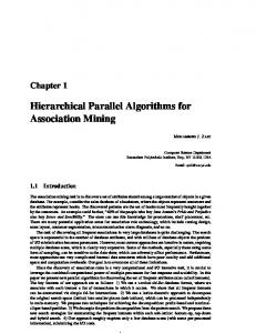
for any ¯i1 , ¯i2 ∈ I and d¯i ∈ D. Lee et al [4], stated the necessary and sufficient conditions for such a transformation T to correctly map a p-nested loop algorithm onto a q-dimensional systolic array, where 1 ≤ q ≤ p −1. They have also described exhaustive and heuristic search methods to determine, respectively, the ¯ and S. Sheu et al [11] describe an algorithm to partition optimal and suboptimal mappings h the index points found on a time hyperplane onto the processors in a message passing system. ¯ = 0. Their method first projects all index points and dependence vectors onto hyperplane hx The projected index points are then grouped along the directions of the projected dependence vectors. The result is that all index points projected onto a point in the same group will not be executed simultaneously. To reduce the communication overhead, the group is made as large as possible. Most methods described in the literature for mapping a computation structure onto an array of processors (or a VLSI array) reduce the problem to an instance of the integer programming optimization. However, the integer programming optimization problem is NP-hard [1]. In this paper, we assume the spacetime representation of an algorithm to be a continuous domain and ¯ termed wavefront, that results in the minimum execution time. determine the time hyperplane h, In our analysis, an algorithm is assumed to be specified using single assignment statements, i.e., each variable is defined no more than once at each index point. To apply the analysis to an algorithm specified using a procedural language, appropriate indexes of the loops surrounding each variable occurrence in the algorithm are needed (a process labeling variables with such indexes is described in [3]). Wavefront scheduling is appropriate for Single Program Multiple Data (SPMD) [10] implementation on distributed memory architecture or for data parallelism on SIMD architectures. SPMD implementation, in general, requires larger parallel granules than SIMD implementation, therefore it is more efficient provided that the computations at each index point are fairly complex (i.e., involve computationally intensive function evaluation). Figure 1 illustrates how the choice of a particular wavefront can affect the performance of an algorithm. A two dimensional array E is to be evaluated on a one-dimensional (logically) processor array. The elements are defined by the following statements (elements that are beyond the array boundary are considered to be zero) ∀(x1 , x2 ) ∈ X :

E[x1 , x2 ] = f (E[x1 − 2, x2 + 2], E[x1 − 4, x2 − 2]) 3

(2)

G’ G

H G"

B (2,-2) H" F’ F"

O A H’

(4, 2)

E"

E’ F

E

Figure 1: Different wavefronts to evaluate array E where the index domain X is [1, n] × [1, n]1 . There are two dependence vectors in this computation, OA ([4,2]) and OB([2,-2]). Since all dependence vectors are on one side of the lines EH, E ′ H ′ and E ′′ H ′′ , all of them are potential wavefronts. However, such a wavefront does not always exist. For example, when data dependences are different at different regions of index domain, there may be no single wavefront with ¯x = c the required property in the entire index domain. All index points lying on hyperplane h¯ can be executed simultaneously, if and only if, values of the array at all the index points ¯ x < c & x¯ ∈ X} X ′ = {¯ x|h¯ are known at this instance of execution, that is, all array elements in an appropriate side of the wavefront have been already evaluated. Two parallel wavefronts form a strip of computation that can be divided among a number of processors for execution. The separation between the wavefronts can be made such that once all packets (containing array elements evaluated by other processors) reach their destination, no more communication is needed to complete the evaluation of all the array elements between the two wavefronts. In fig. 1, EF GH, E ′ F ′ H ′ G′ and E ′′ F ′′ H ′′ G′′ are three such strips. Since EF GH covers a bigger area than E ′ F ′ G′ H ′, computation along this wavefront results in less frequent communication and synchronization. Wavefront EH can be preferred to E ′′ H ′′ for another reason, namely the smaller distance that data must travel (compare projection of OA on E ′′ H ′′ with the projection of OA on EH). Wavefront EH can be partitioned into more sections than E ′′ H ′′ with the similar computation to communication ratio, leading to a higher degree of parallelism. Even if there are no restrictions on the number of available processors, it is not straightforward to determine how the wavefronts should be optimally partitioned and mapped to the processors. Partitioning a wavefront into small sections increases communication time, because most of the input array elements needed to evaluate a particular index point may reside outside the evaluating 1

more conventional definition of this index domain would be a loop nest f or(x1 = 1; x1 ≤ n; x1 + +) f or(x2 = 1; x2 ≤ n; x2 + +) . . ..

4

processor’s local memory. For certain dependence vectors and the sizes of the partitions, input array elements may be quite a few processors away. On the other hand the processors may be underutilized, if a large section of the wavefront is assigned to a single processor. Given a nested loop, algorithms for partitioning the index domain among a number of processors to minimize the total computation time involve solving an integer optimization problem that is NP-hard [8, 14]. In this paper, we discuss polynomial-time algorithms for such partitioning under the simplifying assumption about positions of the index points versus wavefronts. The paper is organized as follows. In section 2 we describe an algorithm for finding the optimum wavefront in a computation defined over two-dimensional arrays executed on a machine with processors interconnected (logically) into one-dimensional array. We describe also an algorithm for optimum partitioning of the wavefront into sections that are assigned to individual processors (after slight modifications, this algorithms can be applied to processor arrays of higher dimensions). Finally, we discuss an algorithm for efficient enumeration of points that are evaluated by a single processor in one computation step. In section 3, we outline the methods for determining good wavefronts for (logically) higher dimensional distributed memory machines. Conclusions and comments on limitation of the presented approach are presented in section 4.

2

Optimum Wavefront for 1-D Interconnected Architectures

Suppose we want to compute an array E defined recursively by equation (2). Such a definition imposes a partial order on the execution of the index points of the array E, and therefore not all elements of the array E can be evaluated simultaneously. In this section we investigate several valid execution orderings of the index points. Our goal is to find the execution ordering that results in the minimum computation time. In this section, we restrict our attention to algorithms involving two dimensional arrays processed on a linear, arbitrary large array of processors. Figure 1 shows the processing of array E. If at some point during execution, E[x1 , x2 ] is known for all index points [x1 , x2 ] located above hyperplane EH, then array E can be evaluated simultaneously at all index points on this hyperplane. Such a hyperplane is termed a wavefront of computation. The direction of computation is perpendicular to the wavefront of computation. A necessary and sufficient condition for a hyperplane to be a wavefront is that all dependence vectors attached to a point on the hyperplane must lie to one side of the wavefront. More formally, if D = {d¯1 , d¯2, . . . , d¯n } is the ¯ · x¯ = c is a wavefront if and only if, either set of all dependence vectors in an algorithm, then h or

¯ x + d¯l ) < h ¯ · x¯, h(¯

∀d¯l ∈ D & ∀¯ x∈X

¯ x + d¯l ) > h ¯ · x¯, h(¯

∀d¯l ∈ D & ∀¯ x∈X

is true (these two conditions are equivalent to the condition in (1)). The direction of computation ¯ ¯ h √h is given by √h· ¯h ¯ in the former case and by − h· ¯h ¯ in the later. Evidently, any line between OB and OA (traversed clockwise) in Figure 1 may be a wavefront, since for these and only these lines are the dependence vectors on one side of the line. We would like to determine the wavefront that results in minimum computation time. 5

Suppose there are n dependence vectors, D = {d¯1 , d¯2 , . . . , d¯n }. The projections of the depen¯ · x¯ = c are given by dence vectors on hyperplane h ¯ · d¯k h ¯ z¯k = d¯k − ¯ ¯ h h·h

∀d¯k ∈ D

Let r + 1 of the dependence vectors extend to the right and l = n − r + 1 to the left. Let zi , i = −l, −l + 1, . . . , −1 and zi , i = 0, 1, 2, . . . , r be the projections of the vectors that extend to the left and to the right, respectively. Without loss of generality we can assume that z−l and zr are the largest projections extended to the left and to the right, respectively, and that z−l ≥ z−l+1 ≥ · · · ≥ z−1 and zr ≥ zr−1 ≥ · · · ≥ z0 (see Figure 2). .

.

.

.

" . ... " S ...  . " " ] S  ". h.. S  " ." . ^.." S . "  " " ." S S  " " ". S S "  " "  >.  yXX" SX "S   X XX " S S " z " . r X."  ... .. S S . " " . .= " ...... " . S " S . 3  3  " . " S " S   . " S . z " l w ." S ".   Pi " S + + . S S S w S

Figure 2: Projection of the dependence vectors on a wavefront Let α (α′ ) and β (β ′ ) denote the minimum and maximum angles made by the dependence vectors with the positive (negative) x-axis. For a wavefront to exist, either β < α + π or β ′ < α′ + π. Without loss of generality we assume in the following that β < α + π. Let θ denote an angle that a wavefront makes with positive x-axis. Depending on the values of α, β the angle θ is in one of the five possible ranges: (i) in (β, α + π), or (ii) in (−π/2, α) ∪ (β, π/2], or (iii) in β − π, α), or (iv) in (−π/2, α − π) ∪ (β − π, π/2], or (v) in (−π/2, α + π) ∪ (β + π, π/2]. By properly redirecting and/or relabeling x and y axes, we can, without loss of generality, restrict our attention just to the first case. Hence, we consider in the further analysis only such angles α, β, θ that −π/2 < β < θ < α + π ≤ π/2. Let c be the communication cost per item (which can either be an individual data element or a packet of data elements, depending on the hardware communication mechanism) and e be the execution cost of one data element. We assume that communication and computation cannot be interwoven and that there is no restriction on the number of available processors. The wavefront execution is characterized by two parameters. The first one, h, defines the distance between two consecutive parallel hyperplanes. All index points within these two hyperplanes are evaluated in one execution step. Such collection of index points is called a computational strip. We require that the partitions of the computational strips allocated to processors are of 6

rectangular shape. The second parameter describing wavefront computation is w, the width of the partition allocated to single processor. Under these assumptions, the execution time of a computation step is E ≤ cC(w) + N(w)e (3)

where C(w) denotes the number of items that needs to be communicated to compute one partition of the computational strip and N(w) stands for the maximum number of index points in the strip. We assume that the computation is synchronized at each wavefront movement and under this assumption the right hand side of the above inequality defines the computation time between wavefront movements. To approximate the maximum number of index points within a partition of a computational strip assume that 0 ≤ θ < π/4 (all other cases with θ ∈ [−π/2, −π/4), [−π/4, 0)and(π/4, π/2) can be analyzed similarly). A strip of thickness cos θ cuts out a unit along the x-axis, hence a partition of length w of this strip contains at most ⌊w cos θ⌋ + 1 index points. Consequently, a partition of length w of a strip with thickness h can contain at most % ! $ h +1 (⌊w cos θ⌋ + 1) cos θ points. Hence

1 1 cos θ + + ) h w cos θ hw Similarly, we can consider a partition of length sin θ that cuts out a unit along the y-axis to arrive at approximation sin θ 1 1 N(w) ≤ hw(1 + + + ) w h sin θ hw that should be used when w ≤ h. Both cases of relation of w to h are analyzed analogously, so without loss of generality we can assume that w > h, then N(w) ≤ hw(1 +

N(w) ≈ hw(1 +

cos θ ) h

(4)

Let’s consider the third factor in (4), i.e. f = 1 + cos θ/h. The thickness of the computational strip is defined by the vector with the shortest projection on the wavefront line. When θ is close to β (α + π) then the vector that makes an angle β (α) with x-axis has this property. In general, h = vh sin(θ − γh ), where vh denotes the length of the dependence vector that defines strip height h, and γh denotes the angle that this vector makes with the x-axis. Hence, f (θ) = 1 +

cos(θ) vh sin(θ − γh )

f ′ (θ) =

− cos(γh ) cos(θ) vh sin2 (θ − γh )

so f is monotonically decreasing with the minimum at the upper boundary of the validity interval. If cos(θ)/h ≥ 1 then h ≤ cos θ and a single wavefront movement cannot reach the next layer of index points. In such case, the number of index points that belongs to different strips in the same wavefront vary widely causing imbalance in the processor load. To avoid such imbalance, we will restrict the possible wavefront angles to the interval [θβ , θα ] in which vectors with angles α and β define strip height h ≥ cos φ. Since, by definition, cos(θβ )/vβ sin(θβ − β) = 1, then 1 θβ = arctan tan β − vβ cos β 7

!

(5)

with the similar definition of θα . If θα < θβ then the optimum wavefront direction should be selected to minimize function f , i.e. at the equal distance between β and α + π, hence θopt = (β + α + π)/2 (since the parallel to this wavefront crosses endpoints of two vectors, the slope of this wavefront is rational). Otherwise, since cos(θ)/h < 1, we can ignore changes in f and approximate N(w) by hw. In the following, we determine the optimum wavefront of computation for two different models of communication: (i) each array element transferred individually, and (ii) array elements transferred in packets.

2.1

Elements Transferred Individually

In this subsection it is assumed that two processors can communicate directly with each other only when they are neighbors. Under this assumption, the minimum width w along wavefront Z that a processor can be allowed to compute is wmin = max(z−l , zr ). For any partition of width w ≥ wmin , the total number of elements communicated from the neighboring partitions can be estimated as follows. Since array elements computed by a neighboring processor are accessed individually, the total number of elements communicated from the processor on the right to the given partition is: Cr (w) = N(z0 ) ∗ (r + 1) + N(z1 − z0 ) ∗ r · · · + N(zr − zr−1 ) Approximating the number of points in the strip fragment of length z by the average density of points in the partition we get N(z) = z ∗ N(w)/w and adding the communication resulting from the left neighbor, we obtain: r N(w) X C(w) = zi w i=−l It follows immediately from the above formula that the communication overhead is the same for all partitions of width w ≥ wmin and therefore to minimize the total computation time we just need to consider the minimum width wmin . The execution time of the single wavefront movement E can now be expressed as (cf. (3)) E ≤ N(w)c f +

Pr

i=−l

w

zi

!

where f = e/c. In order to minimize the total execution time we need to consider the number of wavefront movements. Let the size of the array being computed be X × Y , then L = X| sin θ| + Y cos θ is the length the wavefront needs to traverse and the total computation time is: L LcN(w) T = E≤ h h

Pr

i=−l zi +f w

!



= Lc wf +

r X

i=−l



zi 

(6)

The first factor, L = X| sin θ| + Y cos θ, represents the distance that the wavefront has to traverse to evaluate rectangle X × Y . Since θ ∈ (−π/2, π/2], therefore for θ < 0 the absolute value of the sine has to be taken. 8

The length of projection of vector (xi , yi ) onto the wavefront is |xi cos θ + yi sin θ| and the sum P of the projection lengths is ri=−l |xi cos θ + yi sin θ|. Finally, the length of the partition w is equal to the length of the longest projection of the dependence vectors on the wavefront, i.e. 

w = max |xi cos θ + yi sin θ| i



The smallest index of the vector that defines w will be denoted by imax. Let {γ1 , γ2, . . . , γm }, m ≥ 0 be a sorted list (possibly empty) of those among the following angles that belong to (θβ , θα ): 1. arctan(− xyii ), −l ≤ i ≤ r, 2. π/2, Let γ0 = θβ , and γm+1 = θα . For each range (γj , γj+1), j = 0, 1, . . . , m, expression (6) can be written as (Z sin θ + Y cos θ)(a cos θ + b sin θ) (7) where Z is either X or −X depending on the value of θ, a = f cimax ximax + ni=1 ci xi , b = P f cimax yimax + ni=1 ci yi , and ci ∈ {+1, −1}. The above formula can be rewritten as P

aZ + bY aY + bZ aY − bZ cos(2θ) + sin(2θ) + 2 2 2 Let φ denote an angle such that aY − bZ sin φ = q (a2 + b2 )(Z 2 + Y 2 )

(8)

aZ + bY cos φ = q (a2 + b2 )(Z 2 + Y 2 )

Formula (8) simplifies to

  1 q 2 2 2 2 (a + b )(Z + Y ) sin(φ + 2θ) + aY + bZ 2 q

and because (a2 + b2 )(Z 2 + Y 2 ) ≥ aY + bZ then the minima of the above functions are all negative and hence the minimum of (6) in the range γi ≤ θ ≤ γi+1 is always at either or both boundaries of the range. By simply listing all the angles γi , i = 0, . . . , m + 1 < (r + l + 1)2 and evaluating (6) we can find an optimal angle θ. Let’s consider the example from Figure 1. There are just three angles to consider: θ1 = − arctan 2, θ2 = π/2, θ3 = π/4. Let’s set X = 100, Y = 10, then the corresponding total computation time from equation (6) is T1 /c = 315f + 315, T2/c = 200f + 400, T3/c = 630f + 630, and depending on the value of f , the first or the second angle should be selected (see Figure 3). In the above analysis we assumed that a processor requests the same array element computed by a neighboring processor every time it needs it. However, if a processor saves the received values when they are referred to more than once, the optimum wavefront can be obtained by determining its angle θ that minimizes 



Lc f w + max proji+ + max proji− i

i



where proji+ stands for max(xi cos θ + yi sin θ, 0) and proji− stands for max(−xi cos θ − yi sin θ, 0). The algorithm described above can be easily modified to determine the optimum value of θ in this case. 9

c

c

c

c

c

c

c

c

c

c

c

c

c

c

c

c

c

c

c c c I @ c c c @c c @ u @f u c c c e f e f e f e f e   u f u c c c f e f e f e f e e   c c c c  c

c

c

c

c

c

c

c f e

c f e

c f e

c f e

c f e

c f e

c

c

c

A A cAA cAA c A c A cAA cAA c c  A A   c AAc AAc Ac Ac AAc AAc f c e I A  A@ A A c c A c A c A@Af cAA f cAA f c e e e A@A  u @Af u Af c c AA c AAf c Af c Af c e e e e e AA      AA f uA f c c cAA f c ceA f ce c eA cA e e e  f f  A A  f c c c AAf ce AAf c e Ac Ac A c A e e e f f  A A  c c ce cAA cAA c A c A cA e e  f f f A A   AA AA A A A 

Figure 3: Optimal wavefronts for array E

2.2

Communication Through Packet Passing

Usually, array elements are not passed individually; instead, several of them are grouped together and sent in a single packet. This method is commonly used in the communication model known as block SIMD. In this model, off-processor values required to compute a designated block of parallel code are obtained immediately before the beginning of the block, and all off-processor values generated within the block are communicated immediately after the end of the block [10]. Typically, packets of values are formed for communication and transferred between nonneighboring processors by means of hopping. Under these assumptions, the minimum width of the wavefront partition assigned to a processor can be less than max(z−l , zr ). With too small a width, processors spend less time computing and more time communicating, because less relevant information is available in the local memory. On the other hand, a large width enables processors to spend more time computing between data transfers, resulting in a smaller communication cost. Beyond a certain width, the communication cost does not decrease any further with an increase in the partition width. If the partitions are too large, the available parallelism may not be exploited fully. Selection of the optimal wavefront and the width size of its partitions under the above-mentioned assumptions is discussed below. In figure 2, P (i) represents the i-th processor that computes a width w of the wavefront. The packets being transferred are rectangular, of size ph × pw . The side of the packet parallel to the wavefront is its width, pw , and the side parallel to the direction of wavefront movement is its height, ph . At each communication step ⌈ zp−l ⌉ packets are received by a processor from left. The w processor retains some of these packets for use in the next (or a future) computation step and forwards relevant packets to its right (similarly for the packets obtained from the right). Figure 4 shows a computation with three dependence vectors d1 , d2 and d3 . Let zr be the longest projection on the wavefront of any dependence vector on the right. Since dependence vectors d2 and d3 have the same projection, the packets sent from processor P (n) are saved by processor P (m) for use at times t1 and t3 (for which the wavefronts are shown). The packet at dependence vector d1 is saved by processor P (m) and also sent to the processors at left for their future use (at time t2 ). This example shows that the transfer of all packets generated to the 10

right (left) up to length zr (z−l ) after every computation phase is sufficient for the computation to proceed.

t1 t2

d2 d3

d1

O

t3

zr

P(n)

P(m)

Figure 4: Packet requirements of different processors The number of packets of size p = ph × pw that pass through P (i) while it computes a strip of length ph along the direction of computation is z−l C(w) = w 

&

'

w zr + pw w 

&

'

&

w z−l (mod w) + pw pw

&

zr (mod w) + pw

'

'

(9)

where w is the size of the wavefront partitions assigned to the processors. A corollary of the following theorem gives the smallest value of w that minimizes C(w). Theorem 1 The minimum value of x C(w) = w 

is

l m x p

&

'

&

w x(mod w) + p p

'

. The smallest value of w for which C(w) reaches the minimum is equal to



x

⌈ xp ⌉



.

Proof The proof is performed by case analysis. Case 1: 0 < w ≤ p l m l m l m In this case C(w) = wx ≥ xp , in particular C(p) = xp . Case 2: mp < wj≤k(ml + 1)p , mm > 0 l m w) r C(w) = (m+1) wx + x( mod . Let x = dw+r where 0 ≤ r < w, then C(w) = d(m+1)+ . p p 11

l m

l

m

= d(m + 1). Hence, ⌈ xp ⌉ ≤ C(w). If r = 0 then C(w) = d(m + 1) and we have xp ≤ d(m+1)p p If np < l rm ≤ (n l + 1)p m for l some n, thenm we have C(w) = (m + 1)d + (n + 1). x dw+r Now, p = ≤ d(m+1)p+(n+1)p = d(m + 1) + (n + 1) = C(w). p p Thus,

l m x p

is the minimum of C(w).

We know from case 1 that the smallest w0 that minimizes C(w) satisfies w0 ≤ p, so C(w0 ) = x w

By definition, at the minimum, w0 =



x ⌈x ⌉ p



l m x p

≤

.

, so w0 is the smallest w for which w ≥

x

⌈x ⌉ p

l

x w0

m

.

. Hence, 2

Corollary : The minimum value of z−l C(w) = w 

&

'

w zr + p w 

l

where L = z−l (mod w) and R = zr (mod w) is reaches minimum is max



z−l ⌈

z−l ⌉ p

 

,

zr ⌈ zpr ⌉

&



.

z−l p

'

&

'

&

w L R + + p p p m

+

l

zr p

m

'

. The smallest w for which C(w)

Let’s consider now the expression (3). We assume that the packet height is selected equal to the strip height, i.e., ph = h. The above corollary shows the smallest w that minimizes C(w) in (9) to be less than or equal to pw . Consequently, if w0 minimizes expression (3) then w0 ≤ pw . But for w ≤ pw z−l zr z−l zr zr z−l + ≤ + ≤ C(w) = + +2 w w w w w w Hence, approximating N(w) with wh, we obtain 



c w



M ph

!





E c + we ≤ ≤ ph w 





M ph

!

+ we +

2c ph

(10)

where M = z−l + zr . E/ph is the execution cost (computation cost plus communication cost) per unit length of computation along the direction of wavefront movement. Expression (10) suggests r should be minimized. that to find the optimum wavefront, z−lp+z h z−l + zr P (θ) = min ph

!

=

min

θ∈(θβ ,θα )

"

maxi (proji )+ + maxi (proji )− mini (yi cos θ − xi sin θ)

#

where proji = xi cos θ + yi sin θ, as previously defined. At any angle θ of the wavefront, at most three dependence vectors are needed to determine P . The angles at which the needed vectors change satisfies at least one of the following equations xi cos θ + yi sin θ = xj cos θ + yj sin θ yi cos θ − xi sin θ = yj cos θ − xj sin θ for some 1 ≤ i, j ≤ n, i 6= j. Let {γ1 , . . . , γm } be a sorted list (possibly empty, in which case, similarly as in the previous subsection, we select (β + α + π)/2 as the angle of the optimum 12

wavefront) of all θ from the interval (θβ , θα ) for which the above conditions are satisfied,   i.e.,   xj −xi −yi ′ ′ sorted list of {θij , θij |1 ≤ i, j ≤ n, i 6= j} where θij = arctan yi −yj and θij = arctan xyjj −x i and θij , θij′ ∈ [θβ , θα ]. As done previously, let γ0 = θβ and γm+1 = θα . For each range of angles θ in (γj , γj+1), j = 0, 1, . . . , m we need to find the n dependence vectors (n ≤ 3) that define P . In each of the ranges γj ≤ θ ≤ γj+1, P can be written as P =

a cos θ + b sin θ c cos θ − d sin θ

c cos θ 6= d sin θ

for some constants a, b, c and d. Now, ad + bc ∂P = ∂θ (c cos θ − d sin θ)2

c cos θ 6= d sin θ

At the extrema of P , ad + bc = 0 and P =

a cos θ + b sin θ a = c cos θ − d sin θ c

Thus if ad + bc = 0, P is a constant function. Otherwise P does not have any extremum point within the range and so the minimum is at either of the boundaries, i.e., either at γj or at γj+1. The angle θ, that minimizes P can be obtained by selecting γk such that P (γk ) = min P (θ),

θ ∈ {γ1 , . . . , γm }

Since m is O(n2), the optimum direction of wavefront can be obtained in O(n2 ) time. Once the optimal angle θ is known, all parameters other than w in expression (3) can be calculated. We have seen that the optimum w is less than equal to pw . From (3) we have E = ph

c ph

! 

z−l zr + w w 



From equation (11), the minimum value of w0 =

E ph

s



+ we =

(11)

is obtained at c(z−l + zr ) ph e

Thus the suitable width w of an individual partition is

2.3

c(z−l + zr ) + we ph w

r

c(z−l +zr ) ph e

when w0 ≤ pw and pw otherwise.

Index Point Enumeration

In this section we present an efficient method for enumerating points in a partition assigned to the given processor. As previously, let θ denote the angle that the optimal wavefront makes with the x-axis, h be the height of its strip and w be the length of its partition. Let’s assume also that the index domain contains all integer points {(x, y|0 ≤ x ≤ X, 0 ≤ y ≤ Y )}. The enumeration is very simple when θ = 0 or θ = π/2, i.e., when the optimum wavefront is parallel to one of the axes of the coordinate system; hence we can exclude such cases from further analysis. As 13

demonstrated in the preceding sections, the optimal wavefront and its direction have a rational slope towards the coordinate axes; consequently there are two relatively prime non-zero integers, qy , qx such that: π qy tan(θ + ) = 2 qx Hence, all index points lie on two families of parallel lines given by: yi =

i qx i qy x+ and zi = − x + qx qx qy qy

The boundaries between partitions are cut by some of these lines because the partition thickness is defined by the end-points of the dependence vectors, so wi = wqx is an integer. Similarly, hi = hqy is also an integer. Before starting the main computation, each processor Pj finds its initial points and wi lines on which these points lie. The lines are given by: yjk =

jwi + k qy x+ where k = 0, 1, . . . , wi − 1 qx qx

During the t-th time step, processors evaluate strip contained between the lines zt = −

qx thi hi x+ and zt+1 = zt + qy qy qy (0)

(0)

For each processor Pj and its line yjk a single initial point (xjk , yjk ) is found from the following equations: (0) xjk

=

(

−1 −(jw if j ≥ 0 i+ k k)qy ijmod qxk  j −jwi −k −jwi −k −1 + − − (jwi + k)qy mod qx if j < 0 qy qy (0)

(0) yjk

qy xjk + jwi + k = qx

where qy−1 is an arithmetic reciprocal of qy modulo qx , i.e. qy−1 qy ≡ 1(modqx ) (the well known Euclidian algorithm can be used to find qy−1 efficiently). Additionally, the position of the initial point versus the first wavefront line z0 is set using an equation djkt = qx2 qy (yjk (xjk ) − zt (xjk )) = (qx2 + qy2 )qx xjk + (jwi + k)qx2 − thi qx qy To execute the main computation, the processor Pj runs the code in Figure 5. There are only a few integer arithmetic operations required for each evaluated index point. ~ (−2, −1), OQ(−1, ~ In the example of figure 6, there are three dependence vectors, OP −2) and ~ OR(−1, −3). Using the results of the previous sections we need to consider only four possible wavefronts: hyperplane parallel to the y-axis and hyperplanes that are perpendicular to the ~ , OQ ~ and OR ~ (shown by dashed, solid and dotted lines, respectively, passing through vectors OP O). The sum of the projections of the √ vectors on a wavefront is minimum for the wavefront ~ and the sum is 4/ 5. If there are enough processors available then each perpendicular to OQ 14

/* initialization */ for(k=0;k++;k < wi ) { (0) x[k]=xjk ; (0) y[k]=yjk ; d[k]=(qx2 + qy2 )qx x[k]+(jwi +k)qx2 ; } /* evaluation */ for(t=0;t< tmax ;t++) for(k=0;k < wi;k++) { while(d[k]< 0) { evaluate(x[k],y[k]); x[k]+=qx ; y[k]+=qy ; if (x[k]>X | y[k]>Y) d[k]=(qx2 + qy2 )qx2 tmax ; else d[k]+=(qx2 + qy2 )qx2 ; } d[k]-=hi qx qy ; }

Figure 5: Index Point Enumeration Code √ one can evaluate a partition of width 4/ 5 resulting in maximum parallelism possible with this wavefront. For example, all index points within the dashed lines P P ′ and RR′ can be allocated to a single processor. All points in the rectangle MNLP (which constitutes a partition) are then computed by the assigned processor in one computational step. All points within the rectangle MNP L lie on two families of parallel lines (each consisting of four lines and the lines of one family are perpendicular to the lines of the other). For this example qx = 1, qy = 1, hi = wi = 4. Each line contributes at most one point to each partition. Assuming that the point origin of the coordinates (i.e. the point (0, 0)) coincides with the point P, the coordinates of the initial points and their lines for the marked partition are: (0, 0), y0 = 2x; (1, 1), y−1 = 2x − 1; (1, 0), y−2 = 2x − 2; (2, 1), y−3 = 2x − 3;

3

Higher Dimension

The problem of finding the best wavefront for distributed memory machines becomes much more complicated for higher dimensions. Suppose we are given a set of mutually recursive equations defining a set of three dimensional arrays. In this case the wavefront is a plane which passes through the three dimensional arrays. For one-dimensional distributed memory machines the compiler can easily determine which of the packets should be retained by a particular processor. 15

P’

R’

S M

O

T N

P Q

L R

Figure 6: Determination of the wavefront

Distance vectors

Processor Array

Figure 7: Routing of packets in a two dimensional processor array

16

z

6

  

   C  ′ ′ ′  (Xi , Yi , Zi )          @

      @ Yi P 

 @      

D        

            

    B

 

   

   * y     

 X   

 i A 

 

    -

x

Figure 8: A two dimensional wavefront ABCD, sweeping through a three dimensional array

However, with two-dimensional distributed memory machines, this determination is very difficult. Figure 7 shows an example in which the compiler can determine the specific routing of the packets that will minimize the number of messages (circles denote processors; routing is shown by the dotted line which passes through all the processors that need a particular packet at some point of the execution). If all inverse dependence vectors can be arranged in such a way that elements in each dimension of the dependence vectors form a sorted list, then such a routing of the packets is easy to arrange. However, the authors are not aware of any general method of arranging the inverse dependence vectors in such a manner. A two dimensional wavefront ABCD is shown in figure 8 sweeping through a three dimensional array. The wavefront is tessellated with rectangles. All the index points in each of the rectangles are processed by a distinct processor. As the wavefront sweeps through the array, each of the rectangles sweeps through a parallelepiped. Index points in each of the parallelepiped are computed by a distinct processor. Let the direction cosines2 of a perpendicular to this wavefront be (γ1 , γ2 , γ3). Let (Xi′ , Yi′ , Zi′ ) be a dependence vector and its projection on the wavefront is at point N. The processor computing index point A need to communicate with the processor that computes index point at (Xi′ , Yi′ , Zi′ ). As shown in figure 8, the relative position of the later processor with respect to the former is ~ is perpendicular (Xi , Yi ). The projection of (γ1 , γ2, γ3 ) on the xz-plane is (γ1 , 0, γ3). Since AB to (γ1 , 0, γ3), its direction cosines are γ1 γ3 , 0, − q ) (q 2 2 2 γ1 + γ3 γ1 + γ32

2 Direction cosines of a vector are the cosines of the angles that the vector makes with the positive x-axis, positive y-axis and positive z-axis.

17

D

C Pd

Pc

Pa

Pb

3N      Yi   p6 y P0  ? ? A px l1  Xi 6

l4 l3

B

l2

Figure 9: Necessary data transfers: Processor P0 needs to communicate with processors Pa , Pb , Pc and Pd to compute the rectangle wx × wy assigned to it ~ are Similarly the direction cosines of AD γ2 γ3 , −q ) (0, q γ22 + γ32 γ22 + γ32

N is the projected point of the position vector (Xi′ , Yi′ , Zi′ ), so ~ = (X ′ , Y ′ , Z ′ ) − (X ′ , Y ′ , Z ′ ) · (γ1 , γ2, γ3 ) AN i i i i i i Thus



~ · AB ~ = (X ′ − X ′ · γ1 ) · Γ13 − Z ′′ · Γ31 Xi = AN i i



~ · AD ~ = (Y ′ − Y ′ · γ2 ) · Γ32 − Z ′′ · Γ23 Yi = AN i i

′′ where Γij = √γγ2i+γ 2 , and Z = Zi′ − Zi′ · γ3 . The communication requirement for the processor i

j

P0 computing the rectangle of index points at A is shown in figure 9. Rectangle of size (l1 × l3 ) needs to be communicated from processor Pa to processor P0 . The number of packets of size px × py in this rectangle located at N is &

' &

'

wx − Xi (mod wx ) wy − Yi (mod wy ) · · px py

The relative position of processor Pa with respect to processor P0 is 

 $

Yi Xi , wx wy

%!

So if the packets are not retained by a processor for future use, the total number of packet transferred between neighboring processors Pa and P0 is WXi

·

WYi

·



$

Xi Yi + wx wy

18



%!

m

l

l

m

wy ) wx ) , and WYi = wy −Yi ( mod . where WXi = wx −Xi ( pmod py x Adding all such packet transfers from processors Pa , Pb , Pc and Pd to processor P0 we get the total communication cost as

C(w) = +

n X

i=1 n X i=1

Wxi Wxi

·

Wyi

·

WYi

&

'!

$

%!

Yi Xi + wx wy

·



·





Xi Yi + wx wy 

+ +

n X

WXi

i=1 n X

WXi

i=1

·

WYi

·

Wyi

$

%!

&

'!

·



Yi Xi + wx wy

·



Xi Yi + wx wy

 

(12)

where px and py are the dimensions of the packets, wx and wy the widths of the array that a processor is assigned to compute, [Xi , Yi ] are the co-ordinates l of the projections m l of the i-th m Yi ( mod wy ) Xi ( mod wx ) i i dependence vector on the wavefront. Wx and Wy stands for and , px py respectively. If we ignore the ceiling and floor functions (i.e., ceiling and floor functions are replaced by the identity function), expression (12) reduces to n X

wx wy C(w) = i=1 px py

Xi Yi + wx wy

!

which suggests that to find a good wavefront attempt should be made to minimize ni=1 |Xi|+|Yi |. Let [xi , yi, zi ] 1 ≤ i ≤ n be the dependence vectors and γ1 , γ2 and γ3 denote the direction cosines of the perpendicular to the wavefront, then we would like to find values of γ1 , γ2 and γ3 that minimize P

|(xi − xi · γ1 ) · Γ31 − (zi − zi · γ3 ) · Γ13 | + |(yi − yi · γ2 ) · Γ32 − (zi − zi · γ3 ) · Γ23 | (Γs are as defined before) under the constraint that γ12 + γ22 + γ32 = 1

0 ≤ γ1 , γ2 , γ3 ≤ 1

Further studies are necessary to design an efficient algorithm for determining γ1 and γ2 that satisfy all these conditions.

4

Final Remarks

The problem of finding the optimum wavefront that minimizes total computation time is discussed in this paper for iterative computations over two-dimensional arrays executed on linear or two-dimensional processor arrays. Assuming a continuum of data elements in two-dimensional arrays computed on a linear array of processors, efficient algorithms have been presented to determine the optimum wavefront of computation and the optimum partitioning of the wavefront into sections assigned to individual processors. An O(n2 ) time algorithm (where n is the number of data dependence vectors) for finding the optimum wavefront for one-dimensional processor arrays has been described. In addition, a method for finding a good wavefront for two-dimensional SIMD machines has been presented. In our analysis, we have assumed a continuum of data elements in an array. In reality, arrays are discrete, so the analysis is approximate. For example in mapping a computation onto a linear 19

array of processors, the algorithm provides very good wavefront when z−l and zr , the longest projections (on each sides) of the data dependence vectors on the selected wavefront, are much larger than pw (the length of the packets along the wavefront). The methods described here can be applied to any set of uncoupled recurrence equations. To decrease the communication cost a good alignment of all arrays in the program should be determined first (see [12, 5]). Many methods described in the literature [11, 3, 4, 7] determine the actual mapping of the computation onto the processors, once the wavefront is determined by solving an integer programming optimization problem (see section 1). These algorithms can be used for the wavefronts obtained by our method. When communication is accomplished by means of packet switching, there is evident difficulty in handling packets that are not cut out in parallel to the natural sides of the arrays. How to generate packets of convenient sizes and shapes that can be handled efficiently, once their size and orientation are known, is an interesting topic for further research. There are many open problems in this area. One major issue concerns finding an efficient algorithm to determine a good wavefront when a set of recurrence equations involving m-dimensional arrays are to be computed on an n-dimensional array of processors (m ≥ n).

References [1] M. R. Garey and D. S. Johnson, Computers and Intractability A Guide to the Theory of NP-Completeness, W. H. Freeman and Company, New York, 1979. [2] L. Lamport. “The parallel execution of do loops”, CACM, 17, 1974. [3] P.-Z. Lee and Z. M. Kedem, “Synthesizing Linear Array Algorithms from Nested For Loop Algorithms”, IEEE trans. on Computers, Vol. 37, No. 12, December 1988. [4] P.-Z. Lee and Z. M. Kedem, “Mapping Nested Loop Algorithms into Multidimensional Systolic Arrays,” in IEEE Transactions on Parallel and Distributed Processing, vol 1, no 1, January 1990. [5] J. Li and M. Chen, Index Domain Alignment: Minimizing Cost of Cross-Referencing Between Distributed Arrays, Tech. Rep., Dept. of Comp. Sc., Yale, Univ., YALEU/DCS/TR-725, November 1989. [6] W. L. Miranker and A. Winkler, “Spacetime Representations of Computational Structures,” in Computing Vol 32, No 2, pp. 93-114, 1984. [7] D. I. Moldovan, “Partitioning and Mapping Algorithms into Fixed Size Systolic Arrays,” in IEEE Transactions on Computers, Vol C-35, No 1, pp. 1-12, January 1986. [8] C. D. Polychronopoulos, D. J. Kuck and D. A. Padua, “Utilizing Multidimensional loop Parallelism on Large-Scale Parallel Processor Systems,” in IEEE Transactions on Computers, Vol 38, No 9, pp. 1285-1296, September 1989. [9] S. K. Rao, Regular Iterative Algorithms and their Implementations on a Processor Arrays, Ph. D. Thesis, Dept. of Electrical Engineering, Stanford University, California, 1985. 20

[10] M. Rosing, R. B. Schnabel and R. P. Weaver, Scientific Programming Languages for Distributed Memory Multiprocessors: Paradigms and Research Issues, in Languages, Compilers and Run-Time Environments for Distributed Memory Machines by J. Saltz and P. Mehrotra (eds), Elsevier Science Publishers, 1992. [11] J.-P. Sheu and T.-H. Tai, “Partitioning and Mapping nested Loops on Multiprocessor Systems,” in IEEE Trans. on Parallel and Distributed Systems, vol. 2, No. 4, pp. 430-439, October 1991. [12] B. Sinharoy and B. K. Szymanski, “Complexity Issues of the Alignment Problem and the Closest Vectors in a Lattice”, Technical Report 91-10, Department of Computer Science, Rensselaer Polytechnic Institute, Troy, NY 12180, May 1991. Submitted to IEEE Transactions on Parallel and Distributed Systems. [13] Szymanski, B.K. (edt): Parallel Functional Languages and Environments ACM Press: New York, NY, 1991 [14] C.-M. Wang and S.D. Wang, “Efficient Processor Assignment Algorithms and Loop Transformations for Executing Nested Parallel Loops on Multiprocessors,” in IEEE Transactions on Parallel and Distributed Systems, Vol 3, No 1, pp. 71-82, January 1992.

21