We propose a Finite-Difference Time-Domain (FDTD) method to model the Sagnac effect, which is based on the modified constitutive relation in rotating frame.
Finite-difference time-domain algorithm for modeling Sagnac effect in rotating optical elements Chao Peng, Rui Hui, Xuefeng Luo, Zhengbin Li and Anshi Xu State Key Laboratory on Advanced Optical Communication Systems & Networks, School of Electronics Engineering and Computer Science, Peking University, China
Abstract: Electrodynamics in rotating optical elements has attracted much interest due to its potential application to ultra-sensitive rotating sensing. And it is important to investigate the Sagnac effect in some novel photonic structures for it may lead to a variety of unusual manifestations. We propose a Finite-Difference Time-Domain (FDTD) method to model the Sagnac effect, which is based on the modified constitutive relation in rotating frame. The time-stepping expressions for the FDTD routine are derived and discussed, and the classical Sagnac phase shift along a waveguide is calculated. Further discussions about numerical dispersion, dielectric boundary condition and perfect matched layer (PML) absorbing boundary conditions in the rotating FDTD model are also presented respectively. The theoretical analysis and simulation results prove that the numerical algorithm can analyze the Sagnac effect effectively, and can be applied to general cases with various material properties and complex geometric structures. The proposed algorithm provides a promising systematic tool to study the properties of rotating optical elements, and to accurately analyze, design and optimize rotation sensitive optical devices. © 2008 Optical Society of America OCIS codes: (120.5790) Sagnac effect, (000.4430) Numerical approximation and analysis, (060.2800) Gyroscopes, (140.3370) Laser gyroscopes
References and links 1. U. Leonhardt and P. Piwnitski, “Ultrahigh sensitivity of slow-light gyroscope,” Phys. Rev. A 62, 055801 (2000). 2. A. B. Matsko, A. A. Savchenkov , V. S. Ilchenko and L. Maleki, “Optical gyroscope with whispering gallery mode optical cavities,” Opt. Commun. 233, 107-112 (2004). 3. J. Scheuer and A. Yariv, “Sagnac Effect in Coupled-Resonator Slow-Light Waveguide Structures,” Phys. Rev. Lett. . 96, 053901 (2006). 4. C. Peng, Z. Li, and A. Xu, “Optical gyroscope based on a coupled resonator with the all-optical analogous property of electromagnetically induced transparency,” Opt. Express 15, 3864-3875 (2007). 5. B. Z. Steinberg, “Rotating photonic crystals: A medium for compact optical gyroscopes,” Phys. Rev. E . 71, 056621 (2005). 6. B. Z. Steinberg and A. Boag “Splitting of microcavity degenerate modes in rotating photonic crystals-the miniature optical gyroscopes,” J. Opt. Soc. Am. B . 24, 142-151 (2006). 7. S. Sunada and T. Harayama, “Sagnac effect in resonant microcavities,” Phys. Rev. A 74, 021801 (2006). 8. S. Sunada and T. Harayama, “Design of resonant microcavities: application to optical gyroscopes,” Opt. Express 15, 16245-16254 (2007). 9. C. Peng, Z. Li, and A. Xu, “Rotation sensing based on a slow-light resonating structure with high group dispersion,” Appl. Opt. 46, 4125-4131 (2007). 10. B. Z. Steinberg, J. Scheuer, and A. Boag, “Rotation-induced superstructure in slow-light waveguides with modedegeneracy: optical gyroscopes with exponential sensitivity,” J. Opt. Soc. Am. B 24, 1216-1224 (2007).
#91999 - $15.00 USD
(C) 2008 OSA
Received 25 Jan 2008; revised 21 Mar 2008; accepted 22 Mar 2008; published 1 Apr 2008
14 April 2008 / Vol. 16, No. 8 / OPTICS EXPRESS 5227
11. E. J. Post, “Sagnac Effect,” Rev. Mod. Phys. 39, 475-493(1967). 12. B. Z. Steinberg, A. Shamir, and A. Boag, “Two-dimensional Green’s function theory for the electrodynamics of a rotating medium,” Phys. Rev. E 74, 016608 (2006). 13. T. Shiozawa, “Phenomenological and electron-theoretical study of the electrodynamics of rotating systems,” Proc. IEEE 61, 1694-1702 (1973). 14. J. L. Anderson and J. W. Ryon, “Electromagnetic radiation in accelerated systems,” Phys. Rev. 181, 1765-1775 (1969) 15. J. Van Bladel, “Relativity and Engineering”, Springer, Berlin, (1984) 16. J. P. Berenger, “A perfectly matched layer for the absorption of electromagnetic,” J. Computational Physics 114 185-200 (1994). 17. A. Taflove, “Computational Electrodynamics: The Finite-Difference Time-Domain Method,” Artech House, Boston, (1995). 18. D. S. Katz, E. T. Thiele, and A. Taflove, “Validation and extension to three dimensions of the Berenger PMLabsorbing boundary condition for FD-TD meshes,” Microwave and Guided Wave Letters, IEEE, 4 268-270, (1994). 19. R. Wang, Y. Zheng, and A. Yao “Generalized Sagnac Effect,” Phys. Rev. Lett. 93, 143901 (2004). 20. V. A. Mandelshtam and H. S. Taylor, “Harmonic inversion of time signals,” J. Chem. Phys. 107, 6756-6769 (1997).
1.
Introduction
Recently, electrodynamics in rotating optical elements has attracted much interest due to its potential application to ultra-sensitive gyroscope [1-10]. Several works have pointed out that the Sagnac effect can be observed in arrays of coupled resonator waveguides [3][4], and it also causes mode-splitting in some photonic crystal structures [5][6]. In addition, the Sagnac effect in resonant micro-cavities is studied [7][8], which shows that the cavity rotation causes shifts of the resonant frequencies proportional to the rotation rate if it is larger than a certain value. Research points to the fact that the Sagnac effect leads to a variety of manifestations in some novel photonic structures, which are significantly different compared with the phase shift phenomenon observed in conventional waveguides. The magnitude of the Sagnac effect depends on the light slowing ability of the respective structure [9], allowing even exponentially sensitive rotation sensing [10]. These phenomena may potentially be utilized as highly sensitive gyroscope, and a general approach to model and analyze such phenomena is required. In conventional waveguides, the Sagnac phase shift can be calculated by using an integral over the light path [9]. To analyze a structure’s response in rotation frame, the most intuitive way is to follow the transfer function, whilst taking into account the Sagnac phase shift along each light path [3][4][9]. However, this method depends on some phenomenological parameters, such as the reflection coefficient and the attenuation factor, which are difficult to determine in the designing phase. Additionally, in some scattering mechanism based photonic structures (such as photonic crystal), there is no exact light path, therefore the transfer function method can not describe this kind of Sagnac effect completely. On the other hand, an analytic model for analyzing the Sagnac effect in micro-cavity structures was proposed [5-8]. For single resonant cavity, a wave-dynamical approach can be applied, and a tight-binding approximation assuming weak-coupling between micro-cavities can be used to deal with the case of multiple resonant cavities. This method works well for simple cavities with good symmetries, but it may encounter difficulties for the cavities with complex structures, for which the eigenstate function may not be resolved easily. And because of the approximation, this analytic model may also lead to some other limitations when applied to general cases. Furthermore, the two-dimensional Green’s function theory was proposed for electrodynamics of a rotating medium [12], which represents the response to a point source. It provides a systematic tool for the general study of the spectral properties of rotating systems. However, as a spectral method, it is not convenient for analyzing transient processes. Currently, the three#91999 - $15.00 USD
(C) 2008 OSA
Received 25 Jan 2008; revised 21 Mar 2008; accepted 22 Mar 2008; published 1 Apr 2008
14 April 2008 / Vol. 16, No. 8 / OPTICS EXPRESS 5228
dimensional theory is still being researched on. Numerical algorithms can thus provide a vital tool to accurately analyze, design and optimize a rotation sensitive optical device. In this paper, we develop a Finite-Difference Time-Domain (FDTD) method for the simulation of the Sagnac effect which is based on the modified constitutive relation in rotating frame. This is an ab initio, time domain method which can simulate the Sagnac effect from real physical parameters, such as material property and geometric structure. It can easily be applied to 2D or 3D situations and complex structures, for studying the device’s behavior in a rotating frame. This paper is organized as follows: In Section 2, we present our theory of the FDTD method. We derive and discuss the 2D situation, and obtain the time-stepping expressions for the FDTD routine; In Section 3, the classical Sagnac phase shift along a conventional silicon waveguide is calculated with the light path integral and the FDTD algorithm respectively, in order to verify our theory; Then in Section.4, we discuss the issues about numerical dispersion, dielectric boundary condition and perfect matched layer (PML) absorbing boundary conditions in the rotating FDTD model respectively. Finally in Section 5, a summary of this paper is provided. 2.
Theory of the FDTD algorithm in rotating frame
Assume the medium rotates slowly around a fixed axis at an angular velocity Ω, which satisfies the slow velocity assumption as |ΩR ≪ c|, R is the rotating radius and c is the speed of light in vacuum. As some early works postulated [13][14], the basic physical laws governing the electromagnetic fields are invariant under any coordinate transformation, including a no inertial one. The transformation from the stationary frame to a rotating frame is only manifested by an appropriate change of the constitutive relation . If the rotation is rather slow, no other relativistic effects can be observed. Then up to the first order in velocity the constitutive relations in the rotation frame become [6][13][14][15]: ~D = ε ~E − c−2~Ω ×~r × H ~ ~B = µ H ~ + c−2~Ω ×~r × ~E
(2.1)
And Maxwell’s equations in rotation frame keep their basic forms as:
∂ ~D ~ − J~ = ∇×H ∂t ∂ ~B ~ = −∇ × ~E − M ∂t
J~ = ~Js + σ ~E ~ ~ =M ~ s + σm H M
(2.2)
Where r = xxˆ + zˆz + zˆz, ~Ω = zˆΩ. The derivation can be started with Eq. 2.1 and Eq. 2.2. As Ω is assumed varying slowly, Ω = const, ∂ Ω/∂ t = 0. And the axis is fixed in rotation frame, which leads to ∂~r/∂ t = 0.Thus, we get:
∂ Hx ∂t ∂ Hy ∂t ∂ Hz ∂t ∂ Ex ∂t ∂ Ey ∂t #91999 - $15.00 USD
(C) 2008 OSA
= = = = =
1 ∂ Ey ∂ Ez ∂ Ez − − (Msx + σm Hx ) − c−2 xΩ ] [ µ ∂z ∂y ∂t 1 ∂ Ez ∂ Ex ∂ Ez − − (Msy + σm Hy ) − c−2 yΩ ] [ µ ∂x ∂z ∂t ∂ Ey 1 ∂ Ex ∂ Ey ∂ Ex − − (Msz + σm Hz ) + c−2 yΩ + c−2 xΩ ] [ µ ∂y ∂x ∂t ∂t 1 ∂ Hz ∂ Hy ∂ Hz − − (Jsx + σ Ex ) + c−2 xΩ ] [ ε ∂y ∂z ∂t ∂ Hz 1 ∂ Hx ∂ Hz [ − − (Jsy + σ Ey ) + c−2 yΩ ] ε ∂z ∂x ∂t
(2.3) (2.4) (2.5) (2.6) (2.7)
Received 25 Jan 2008; revised 21 Mar 2008; accepted 22 Mar 2008; published 1 Apr 2008
14 April 2008 / Vol. 16, No. 8 / OPTICS EXPRESS 5229
∂ Ez ∂t
=
∂ Hy 1 ∂ Hy ∂ Hx ∂ Hx [ − − (Jsz + σ Ez ) − c−2 yΩ − c−2 xΩ ] ε ∂x ∂y ∂t ∂t
(2.8)
For the 2D situation, all partial derivatives of the fields with respect to z should be zero, thus Eq. 2.3-2.8 can be further simplified. We consider a free propagation case in which there is no electronic or magnetic source, as a result, the terms related to J and M vanish. From these modified Maxwell’s equations above, it is noticed that the electromagnetic fields can still be divided into two independent groups: Ex , Ey , Hz for TE modes and Hx , Hy , Ez for TM modes. Compared with the ordinary form of Maxwell’s Equations, some extra terms which represent the Sagnac effect are induced, whose magnitudes are in the order of c−2 and proportional to rotation velocity. Without loss of generality, we focus the discussion on TE mode, and ∂ Ex /∂ t, ∂ Ey /∂ t, ∂ Hz /∂ t can be resolved with discarding the c−4 terms, then it leads to:
∂ Ex σ + Ex ∂t ε ∂ Ey σ + Ey ∂t ε ∂ Hz σm + Hz ∂t µ
1 ∂ Hz c−2 xΩ ∂ Ex ∂ Ey + − − σm Hz ) ( ε ∂y εµ ∂y ∂x 1 ∂ Hz c−2 yΩ ∂ Ex ∂ Ey = − ( + − − σm Hz ) ε ∂x εµ ∂y ∂x 1 ∂ Ex 1 ∂ Ey c−2 yΩ ∂ Hz − + − σ Ey ) = (− µ ∂y µ ∂x εµ ∂x c−2 xΩ ∂ Hz + − σ Ex ) ( εµ ∂y
=
(2.9) (2.10)
(2.11)
Here, Hz can be split to two components Hzx and Hzy as Berenger’s solution for the perfect matched layer (PML) [16], therefore, Eq. 2.11 can be written as:
∂ Hzx σm + Hzx ∂t µ ∂ Hzy σm + Hzy ∂t µ
1 ∂ Ey c−2 yΩ ∂ Hz + − σ Ey ) (− µ ∂x εµ ∂x 1 ∂ Ex c−2 xΩ ∂ Hz + − σ Ex ) ( µ ∂y εµ ∂y
= −
(2.12)
=
(2.13)
Fig. 1. 2D Yee lattice
In order to discretize Maxwell’s equations, the FDTD model stores field components for different grid locations and time steps. The Yee lattice is widely used in conventional FDTD #91999 - $15.00 USD
(C) 2008 OSA
Received 25 Jan 2008; revised 21 Mar 2008; accepted 22 Mar 2008; published 1 Apr 2008
14 April 2008 / Vol. 16, No. 8 / OPTICS EXPRESS 5230
algorithms [17], as Fig. 1 shows. E, H components are interleaved at intervals ∆x, ∆y in space. The Hz components are located at point i, i+1, · · · , and surrounded by Ex , Ey components which are located at point i + 1/2, i + 3/2, · · · . On the other hand, the leapfrog scheme is also commonly used [17]. The temporal locations of the E and H components are interleaved at intervals of half time-step (∆t/2). H components are calculated at time-step n from the previous field components, and E components are calculated at time-step n + 1/2. Equation 2.9-2.13 are ready for discretization now. This discretization is based on the Yee lattice and leapfrog scheme, using exponential stepping, as described by Katz, et al.[18], and following Yee’s notations [17], we obtain: n+1/2
Ex |i, j+1/2
n−1/2
= exp(−σi, j+1/2 ∆t/εi, j+1/2 )Ex |i, j+1/2 − +
n+1/2
Ey |i+1/2, j
1 − exp(−σi, j+1/2 ∆t/εi, j+1/2 ) c−2 xΩ ∂ Ex ∂ Ey − − σm Hz )|ni, j+1/2 ( σi, j+1/2 µi, j+1/2 ∂ y ∂x
n−1/2
= exp(−σi+1/2, j ∆t/εi+1/2, j )Ey |i+1/2, j − −
Hzx |n+1 i, j
= exp(−σm;i, j ∆t/µi, j )Hzx |ni, j −
+
(2.15)
1 − exp(−σm;i, j ∆t/µi, j ) n+1/2 Ey |i, j ∆xσm;i, j
1 − exp(−σm;i, j ∆t/µi, j ) c−2 yΩ ∂ Hz n+1/2 (− − σ Ey )|i, j σm;i, j εi, j ∂x
= exp(−σm;i, j ∆t/µi, j )Hzy |ni, j −
(2.14)
1 − exp(−σi+1/2, j ∆t/εi+1/2, j ) n Hz |i+1/2, j ∆xσi+1/2, j
1 − exp(−σi+1/2, j ∆t/εi+1/2, j ) c−2 yΩ ∂ Ex ∂ Ey ( − − σm Hz )|ni+1/2, j σi+1/2, j µi+1/2, j ∂ y ∂x
−
Hzy |n+1 i, j
1 − exp(−σi, j+1/2 ∆t/εi, j+1/2 ) n Hz |i, j+1/2 ∆yσi, j+1/2
(2.16)
1 − exp(−σm;i, j ∆t/µi, j ) n+1/2 Ex |i, j ∆yσm;i, j
1 − exp(−σm;i, j ∆t/µi, j ) c−2 xΩ ∂ Hz n+1/2 − σ Ex )|i, j ( σm;i, j εi, j ∂y
(2.17)
Equation 2.14-2.17 are the time-stepping expressions for FDTD routine. They are valid in the whole computational region, including the PML region. For the free propagation case, if (σ , σm ) = 0, the exponential term should be treated carefully, as in lim
σ →0
1 − exp(−σm ∆t/mu) 1 − exp(−σ ∆t/ε ) = ∆t/ε , lim = ∆t/µ σm →0 σ σm
(2.18)
However, there is a problem when applying the Yee lattice to the FDTD algorithm we proposed, that is not all of the required field components are stored in the grid. Such as Hz |ni, j+1/2 , which is required by Eq. 2.14, but it is not stored at point (i, j + 1/2). A way to resolve the problem is to approximately express it as (Hz |ni, j + Hz |ni, j+1 )/2, which are all readily available. n+1/2
n+1/2
This strategy can also be applied to Ex |i, j and Ey |i, j . Using leapfrog scheme, Hzx and Hzy are stored at time-step n, Ex and Ey are stored at timestep n + 1/2. This scheme also leads to another problem that some field components are not n+1/2 available at certain temporal locations. For instance, to calculate Ex |i, j+1/2 by Eq. 2.14, we need #91999 - $15.00 USD
(C) 2008 OSA
Received 25 Jan 2008; revised 21 Mar 2008; accepted 22 Mar 2008; published 1 Apr 2008
14 April 2008 / Vol. 16, No. 8 / OPTICS EXPRESS 5231
∂ Ex /∂ y, ∂ Ey /∂ x at time-step n, but they are not available in the computer’s memory. However, an extrapolation method can be applied to estimate their values, which is based on the values at previous time steps. For a simple linear extrapolation, only the values at time step n − 1/2 and n − 3/2 are required. We can extend this extrapolation to higher orders, if higher accuracy is required. At any given time step, the centered finite-difference (central-difference) expressions are used for the spatial and temporal derivatives that are second-order accurate in space and time increment [17]. For instance, ∂ Hz /∂ y|ni, j , which is required by Eq. 2.17, can be expressed as (Hz |ni, j+1 − Hz |ni, j−1 )/2∆y. But it doesn’t work for the cells at the boundary because they can not be “centered”. We also need an extrapolation method to estimate their values, which are based on the spatial derivatives in internal cells. At least two adjacent internal cells are required for the simplest extrapolation, and more cells may be needed for some sophisticated extrapolation methods. To extend the analysis to the 3D situation, substitute Eq. 2.8 to Eq. 2.3 and 2.4, and discard the c−4 terms, then the temporal differentials ∂ Hx /∂ t and ∂ Hy /∂ t can be expressed by spatial differentials. We can repeat this procedure and obtain six equations with temporal differentials on one side and spatial differentials on the other side. Then by discretizing these equations, the time-stepping equations for FDTD routine can be obtained. The discussion about the extrapolation technique can be also extended to the 3D case. 3.
Modeling 2D rotating waveguide by the FDTD algorithm
The Sagnac effect shows that, when an electromagnetic wave propagates in a moving medium, it accumulates additional phase shift compared with a wave propagating in a stationary medium [11]. This phase shift depends on the scalar product of the wave propagating direction and the velocity vector of the medium, as in ∆φ = 2π~v · ∆~l/cλ
(3.1)
A well investigated configuration is that of two waves counter propagating along a circular path in rotating medium. The total phase shift can be calculated with an integral over the light H path as ∆φ = 4cλπ l ~v · ∆~l . It is well known that this total phase shift, a) does not depend on the shape of the light path; b) does not depend on the location of the center of rotation; c) does not depend on the presence of commoving refracting medium in the light path [11]. Actually, R. Wang et al [19] point out that the Sagnac effect does not only exist in circular motion, but any moving path contributes to the total phase shift. So Eq. 3.1 is the basic differential form to describe the Sagnac effect along a light path. Based on the FDTD model, it is expected that Eq. 3.1 can be verified. Our simulation model is set up for a 2D silicon dielectric waveguide, as Fig. 2 shows. A continuous point source is put into the waveguide, and the waveguide’s width is tailored so that only single mode can propagate. In fact, multi-modes may still exist near the source, because those modes, which cannot propagate, do not decay as fast. However, theoretically, Eq. 3.1 should still hold in spite of the multi-modes. Unlike most of other FDTD simulations, the phase information is much more interesting for studying the Sagnac effect, compared with the field amplitude. For the position at (i, j), the value of the field component at every time step can be recorded as f (n∆t), and the spectrum F(ω ) for this time domain signal can be calculated by Fourier transformation, as R N−1 f (n∆t)e− jω n∆t ∆t. The phase angle of the complex frequency F(ω ) = 0N∆t f (t)e− jω t dt ≃ ∑n=0 represents the phase information. Thus the phase difference between two positions A and B can be obtained from the respective spectrum immediately, as ∆φ = arg(FA (ω )) − arg(FB (ω )). #91999 - $15.00 USD
(C) 2008 OSA
Received 25 Jan 2008; revised 21 Mar 2008; accepted 22 Mar 2008; published 1 Apr 2008
14 April 2008 / Vol. 16, No. 8 / OPTICS EXPRESS 5232
H 1
H 12
H 1
half-width
Fig. 2. The field diagram for Hz The simulation is setup for a silicon waveguide. We use 2-order Berenger PML boundary condition. The simulation condition is set to: The number of grid in x direction: Nx = 100 The number of grid in y direction: Ny = 50 The number of grid for PML layer: Nb = 80 The space differentials: ∆x = ∆y = λ /100 The courant stability factor: S = 0.5 The wavelength of the point source: 1.550µ m The position of the point source: x = 5, y = 25 Half-width of the waveguide: halfwidth= 10 Relative permittivity of the waveguide: ε = 12
Indeed, how to extract the unknown frequencies and phases from discrete time signals, sometimes called ”harmonic inversion”, is a well investigated problem and various algorithms are proposed to resolve it [20]. Generally, the velocity can be resolved into two orthogonal directions, we notate Vx = −yΩ and Vy = xΩ. Because the Sagnac phase shift is proportional to the scalar product of the wave propagating direction and the velocity, thus Vx 6= 0 leads to an additional phase shift, and it is a constant when Vy varies. It is also well known that the waveguide dispersion can in no way influence the magnitude of the Sagnac effect. Different width and refractive index of the waveguide may cause different propagation modes, but the Sagnac phase shift should be unchanging. The Sagnac phase shift along the waveguide can be written as ∆φsagnac = ∆φrotating − ∆φstationary . We calculate it for a series of positions along the center of the waveguide, and the results are plotted in Fig. 3(a)-3(c). The simulation results agree well with Eq. 3.1, which proves that the Sagnac phase shift is a constant regardless of the velocity in the perpendicular direction to the waveguide, the width of the waveguide and the refractive index of the material. These exactly confirm the theory’s assumptions. Therefore the proposed FDTD algorithm can effectively model the classical Sagnac effect along the waveguide. Thus it is believed that: this algorithm can be applied to many other photonic structures with various material properties and #91999 - $15.00 USD
(C) 2008 OSA
Received 25 Jan 2008; revised 21 Mar 2008; accepted 22 Mar 2008; published 1 Apr 2008
14 April 2008 / Vol. 16, No. 8 / OPTICS EXPRESS 5233
theoretic result
1.8
Vy=0
Vx=2m/s
Vy=5
1.6
Vx=1m/s
1.4
-8
Sagnac phase shift(10 rad)
Vy=-5
1.2
1.0
0.8
0.6
0.4
0.2
0.0 0
10
20
30
40
50
60
70
80
distance( x)
(a) theoretic result
1.8
half-width=10
Vx=2m/s
half-width=8
1.6
-8
Sagnac phase shift(10 rad)
half-width=12 1.4
Vx=1m/s
1.2
1.0
0.8
0.6
0.4
0.2
0.0 0
10
20
30
40
50
60
70
80
distance( x)
(b) 1.8
theoretic result =12
1.6
Vx=2m/s
=10
Vx=1m/s
-8
Sagnac phase shift(10 rad)
=14 1.4
1.2
1.0
0.8
0.6
0.4
0.2
0.0 0
10
20
30
40
50
60
70
80
distance( x)
(c) Fig. 3. The Sagnac phase shift vs. distance. The reference position is x = 15 and y = 25. The solid line is the theoretic result from Eq. 3.1, and the marked points are simulation results from the FDTD program. (a) halfwidth= 10; ε = 12;Vy = −5, 0, 5m/s(b) halfwidth= 8, 10, 12; ε = 12;Vy = 0m/s(c) halfwidth= 10; ε = 10, 12, 14;Vy = 0m/s #91999 - $15.00 USD
(C) 2008 OSA
Received 25 Jan 2008; revised 21 Mar 2008; accepted 22 Mar 2008; published 1 Apr 2008
14 April 2008 / Vol. 16, No. 8 / OPTICS EXPRESS 5234
complex geometric structures, to study their behavior in rotating frame. An extrapolation method is applied to obtain the field components which are not available in the computer’s memory. The accuracy of the model certainly depends on the extrapolation accuracy. A two point linear extrapolation technique is used in our simulation. This is a very simple implementation, and other sophisticated extrapolation algorithms can be applied to achieve higher accuracy. It is necessary to point out that, computational mesh setting and the PML layer setting are subtle for the FDTD algorithm. The numerical dispersion which is caused by the discrete gridding may bring some negative impacts to the Sagnac phase shift. We present an analysis about what is the contribution of rotation to the numerical dispersion of FDTD algorithm in Section.4.1. On the other hand, the PML absorption boundary insures theoretically no wave reflection [16][17], but the additional term which represents the Sagnac effect may break this law. To what extent the absorbing boundary conditions are appropriate for the new set of equations Further discussions about the PML boundary are presented in Section.4.3. 4. 4.1.
Analysis and discussion about the FDTD model in rotating frame Numerical dispersion and stability
The Sagnac effect in its basic form is manifested as a phase accumulation. However, the numerical dispersion which is caused by the discrete gridding will also induce non-physical phase error, and it may bring some negative impacts to the FDTD model. Therefore, it is necessary to investigate the numerical dispersion and stability applicable to the FDTD model in rotating frame. The discussion can be started with the modified Maxwell’s equations Eq. 2.9-2.13. For simplicity, assume the FDTD modeling space is filled with homogeneous material having no variation of ε , µ with position in the grid, and there are no magnetic or electric loss, then the system yields 1 ∂ Hz Vy ∂ Ex ∂ Ey + 2( − ) (4.1) ε ∂y n ∂y ∂x 1 ∂ Hz Vx ∂ Ex ∂ Ey = − − 2( − ) (4.2) ε ∂x n ∂y ∂x 1 ∂ Ex 1 ∂ Ey Vx ∂ Hz Vy ∂ Hz = − + 2 + 2 (4.3) µ ∂y µ ∂x n ∂x n ∂y √ Here Vx = −yΩ and Vy = xΩ, n = εr µr is the refractive index of the material. Based on the equations above, the finite-difference expressions for this TE case can be obtained. Such as Eq. 4.1, it becomes:
∂ Ex ∂t ∂ Ey ∂t ∂ Hz ∂t
n+1/2
=
n−1/2
Ex |i, j+1/2 − Ex |i, j+1/2 ∆t
= +
n n 1 Hz |i, j+1 − Hz |i, j ε ∆y n n n n Vy Ex |i, j+1 − Ex |i, j Ey |i+1/2, j+1/2 − Ex |i−1/2, j+1/2 ( − ) (4.4) n2 ∆y ∆x
As mentioned in Section.2, some field components may not be available in computer’s memory because of the spatial and temporal grid discretization under certain algorithm. An extrapolation method is suggested to obtain these field components. If a fine enough extrapolation is applied, Eq. 4.4 is valid with good enough accuracy. Next,we consider a plane, monochromatic, traveling-wave solution in rotating frame, as F|nI,J = F0 exp[ j(ω ∆t − k˜x I∆x − k˜y J∆y)] where F = Ex , Ey , Hz #91999 - $15.00 USD
(C) 2008 OSA
(4.5)
Received 25 Jan 2008; revised 21 Mar 2008; accepted 22 Mar 2008; published 1 Apr 2008
14 April 2008 / Vol. 16, No. 8 / OPTICS EXPRESS 5235
where ω is the wave angular frequency, k˜x and k˜y are the x- and y-components of the numerical wavevector. It should be noticed that the numerical wavevector here contains the contribution from the Sagnac effect, therefore it is slightly different with the wavevector in the stationary frame. The basic procedure for the numerical dispersion analysis involves substitution of the plain wave solution Eq. 4.5 into the finite-difference expressions Eq. 4.4, after simplification, it leads that Ex0 = −
∆tHz0 sin (k˜y ∆y/2) ∆tVy Ex0 sin (k˜y ∆y/2) ∆tVy Ey0 sin (k˜x ∆y/2) · − 2 · + 2 · ε ∆y sin (ω ∆t/2) n ∆y sin (ω ∆t/2) n ∆x sin (ω ∆t/2)
(4.6)
Eq. 4.2,4.3 can be treated similarly, Ey0 =
∆tHz0 sin (k˜x ∆x/2) ∆tVx Ex0 sin (k˜y ∆y/2) ∆tVx Ey0 sin (k˜x ∆x/2) · + 2 · − 2 · ε ∆x sin (ω ∆t/2) n ∆y sin (ω ∆t/2) n ∆x sin (ω ∆t/2)
Hz0 = −
∆tEx0 sin (k˜y ∆y/2) · µ ∆y sin (ω ∆t/2)
+ −
(4.7)
∆tEy0 sin (k˜x ∆x/2) · µ ∆x sin (ω ∆t/2) ∆tVx Hz0 sin (k˜x ∆x/2) ∆tVy Hz0 sin (k˜y ∆y/2) · − 2 · (4.8) n2 ∆x sin (ω ∆t/2) n ∆y sin (ω ∆t/2)
Upon substituting Ex0 of Eq. 4.6, Ey0 of Eq. 4.7 into Eq. 4.8, we obtain k˜y ∆y 2 k˜x ∆x 2 1 1 ω ∆t 2 n sin( )] = [ sin( )] + [ sin( )] c∆t 2 G∆x 2 G∆y 2 ∆tVx sin (k˜x ∆x/2) ∆tVy sin (k˜y ∆y/2) + · where G = 1 + 2 · n ∆x sin (ω ∆t/2) n2 ∆y sin (ω ∆t/2) [
(4.9)
Equation 4.9 is the general numerical dispersion relation of the FDTD model in rotating frame. Compared with the numerical dispersion relation in the stationary frame[17], only a factor of G is induced, and it is related to the Sagnac effect. To obtain the ideal physical dispersion relation in rotating frame, we consider a physical plane wave propagating in a homogenous lossless rotating medium. Because of the rotation, the Sagnac effect induces an extra phase shift, then the plane wave can be written as: F|nI,J = F0 exp[ j(ω ∆t − kx I∆x − ky J∆y − ∆φ )]
(4.10)
Here kx , ky are the wavevectors in the stationary frame without taking accout the Sagnac effect; ∆φ presents the Sagnac effect shift, as Eq. 3.1 shows, which depends on the scalar product of the wave propagating direction and the velocity vector of the medium, then it can be rewritten as: ∆φ
= =
2π ~k ~ ~k ~ ( · V )( · ∆r) λ c |k| |k| 1 (kxVx + kyVy )(kx I∆x + ky J∆y) n2 ω
(4.11)
From Eq. 4.10 and 4.11, the wavevector which contains the contribution from the Sagnac effect in Eq. 4.5 yields 1 1 k˜x = G0 kx , k˜y = G0 ky where G0 = (1 + 2 kxVx + 2 kyVy ) n ω n ω #91999 - $15.00 USD
(C) 2008 OSA
(4.12)
Received 25 Jan 2008; revised 21 Mar 2008; accepted 22 Mar 2008; published 1 Apr 2008
14 April 2008 / Vol. 16, No. 8 / OPTICS EXPRESS 5236
In contrast to the numerical dispersion relation of Eq. 4.9, the ideal dispersion relation can be obtained from (nω /c)2 = (kx )2 + (ky )2 , and Eq. 4.12, it is k˜y k˜x nω 2 (4.13) ) = ( )2 + ( )2 c G0 G0 Equation 4.9 and Eq. 4.13 show that the two dispersion relations are identical in the limit as ∆x, ∆y, ∆t approach zero. Qualitatively, this suggests that if fine enough gridding is chosen, the impact of numerical dispersion can be reduced to any desired degree. The numerical wavevector in rotating medium is proportional to the numerical wavevector in stationary frame with the factor G, which represents the Sagnac effect numerically. So that the Sagnac phase shift will not be submerged in the numerical phase error due to the algorithm’s nature. For the FDTD model in stationary frame, the numerical waves in a 2D/3D Yee lattice have a propagation velocity which is dependent upon the direction of wave propagation. This is also true for the FDTD algorithm in rotating frame. From the expression of G, it is apparent that the numerical wave experiences an anisotropic Sagnac phase shift. These errors represent a fundamental limitation of all grid-based Maxwell’s equations’ algorithms, and can be troublesome when modeling electronically large structures. Further work to improve the computation accuracy is required. (
4.2.
Dielectric boundary conditions in rotating frame
Another important question is to what extent the boundary conditions at a dielectric material boundary are preserved in rotating frame. For non-rotating cases, the boundary conditions can be derived directly from the integral form of Maxwell’s equations focusing on a small region at an interface of two media. As we discussed in Section.2, the Maxwell’s equations governing the electromagnetic fields are invariant in rotating frame, but an appropriate change of the constitutive relation is induce to represent the Sagnac effect. Because the integral form of Maxwell’s equations is independent of the constitutive relation, the basic forms of dielectric boundary conditions are also invariant in rotating frame, as ~2 − D ~ 1) = Σ ~n · (D ~2 − E ~1 ) = 0 ~n × (E
~2 − B ~1 ) = 0 ~n · (B ~2 − H ~ 1) = K ~ ~n × (H
(4.14) (4.15)
However, if it is necessary, the modified constitutive relation should be applied to the boundary conditions to calculate a rotating model. For instance, ~ ~n · ~D =~n · (ε ~E) − c−2~n · (~Ω ×~r × H) −2 ~ ~ + c ~n · (Ω ×~r × ~E) ~n · ~B =~n · (µ H)
(4.16) (4.17)
Fortunately, in 2D geometries rotation case with ~Ω = Ωˆz, the boundary conditions can be further simplified. Form Eq. 4.15, it is notice that the continuity of the tangential E and H fields still preserved across the dielectric interface. If ~Ω is in the z-direction, for a small region at the media interface, I
~ · d~S = 0; (~Ω ×~r × H)
I
(~Ω ×~r × ~E) · d~S = 0;
(4.18)
so that Eq. 4.14 can be written as: ~n · (ε~E2 − ε~E1 ) = Σ
~n · (µ~H2 − µ~H2 ) = 0
(4.19)
They are the same as the boundary conditions in the stationary frame. The 2D geometries rotation does not affect boundary conditions at the dielectric interface. With this result, those well tested legacy codes for modeling stationary structures can also be extended to dealing with rotating structures, with the new set of the time-stepping equations as Eq. 2.14-2.17. #91999 - $15.00 USD
(C) 2008 OSA
Received 25 Jan 2008; revised 21 Mar 2008; accepted 22 Mar 2008; published 1 Apr 2008
14 April 2008 / Vol. 16, No. 8 / OPTICS EXPRESS 5237
4.3.
Absorbing boundary conditions (ABC) in rotating FDTD model
Recall that the ABCs used in the rotating FDTD model were originally developed for nonrotating cases. It is also necessary to consider whether they are appropriate for the new set of equations of rotating medium. The PML absorption boundary insures theoretically no wave reflection [16][17], but the additional term which represents the Sagnac effect may break this law. However, qualitatively, the magnitude of the rotating related term is in the order of c−2 , thus its influence on the validity of the PML boundary condition may be limited. To discuss the PML absorbers in rotating medium analytically, consider the time-harmonic forms of Eq. 2.3-2.8 in a rotating medium, where no electronic or magnetic source exist, it leads to: jωε sy E˜x jωε sx E˜y jω µ s∗x H˜zx jω µ s∗y H˜zy
∂ H˜z + jω c−2Vy H˜z ∂y ∂ H˜z − jω c−2Vx H˜z = − ∂x ∂ E˜y − jω c−2Vx E˜y = − ∂x ∂ E˜x − jω c−2Vy E˜x = ∂y
=
(4.20) (4.21) (4.22) (4.23)
Here the notations are simplified by introducing the variables sw = 1 + σw / jωε ; s∗w = 1 + σw∗ / jω µ ; where w = x, y
(4.24)
To evaluate the ABCs, the basic procedure is to derive the plain-wave solution in the rotating PML medium and calculate the field reflection across the media interface. We consider a TE-polarized wave incident from the lossless medium half-space (Region 1, x < 0), onto the material half-space having the eletric conductivity σ and magnetic loss σ ∗ (Region 2, x > 0). Substituting the expressions for ∂ E˜y /∂ x and ∂ E˜x /∂ y form Eq. 4.20,4.21 into Eq. 4.22,4.23, we obtain the wave-equation in rotating medium: 1 ∂ 2 H˜z jω c−2Vx ∂ H˜z jω c−2Vy ∂ H˜z 1 ∂ 2 H˜z + ∗ + + + ω 2 ε µ H˜z = 0 2 ∗ sx sx ∂ x sy sy ∂ y 2 sx s∗x ∂x sy s∗y ∂y
(4.25)
this wave-equation support the solution: H˜z = H0 exp(− j
q p sx s∗x k˜x x) · exp(− j sy s∗y k˜y y)
(4.26)
with the dispersion relation q p 2 2 k˜x + k˜x − 2ω c−2Vx k˜x / sx s∗x − 2ω c−2Vy k˜y / sy s∗y = (nω /c)2 Then, from Eq. 4.28, 4.20, 4.21, all fields in Region 2 can be obtained: √ ˜ x) · exp(− jpsy s∗y k2y ˜ y) H0 τ · exp(− j s2x s2 ∗x k2x H˜2z = r √ s ∗ k˜ V ˜ x) · exp(− jps2y s2 ∗y k2y ˜ y) E˜2x = H0 τ [− ωε2y2 s22yy + ε s y c2 ] · exp(− j s2x s2 ∗x k2x 2 2y q ∗ p √ ˜ s2 x k2x Vx ∗ ˜ ∗ ˜ E˜2y = H0 τ [ ωε s2x − ε s c2 ] · exp(− j s2x s2 x k2x x) · exp(− j s2y s2 y k2y y) 2 2 2x
#91999 - $15.00 USD
(C) 2008 OSA
(4.27)
(4.28) (4.29) (4.30)
Received 25 Jan 2008; revised 21 Mar 2008; accepted 22 Mar 2008; published 1 Apr 2008
14 April 2008 / Vol. 16, No. 8 / OPTICS EXPRESS 5238
We know that the PML formulation represents a generalization of normally modeled physical media. If σx = σy = 0 and σx∗ = σy∗ = 0, it reduces to a lossless homogenous medium. In this case, the above dispersion relation Eq. 4.27 consists with Eq. 4.13. Therefore, in Region 1, the total field are given by H˜1z = E˜1x =
H0 [1 + Γ exp(2 jk1x )] · exp(− jk1x x) exp(− jk1y y)
V + ε cy2 ] · exp(2 jk1x )] · exp(− jk1x x) exp(− jk1y y) 1 k1 x Vx H0 [1 − Γ exp(2 jk1x )][ ωε ] · exp(2 jk1x )] · exp(− jk1x x) exp(− jk1y y) − ε1 c2 1
k1 y H0 [1 + Γ exp(2 jk1x )][− ωε 1
E˜1y =
(4.31) (4.32) (4.33)
where Γ and τ is the H-field reflection and transmission coefficients. As we discussed in Section.4.2, the dielectric boundary conditions still hold for 2D rotating medium, thus the tangential E and H fields must be preserved across the x = 0 interface. For non-rotating cases, the PML-ABC requires sy = s∗y = 1, sx = s∗x , ε1 = ε2 , µ1 = µ2 , or equivalently σy = 0 = σy∗ , σx /ε1 = σx∗ /µ1 . Apply them to Eq. 4.28-4.33, it is noticed that the phase-matching condition kx1 = kx2 , ky 1 = ky 2 still hold for the rotating case. Further, we derive the H-field reflection and transmission coefficients: r r k1x Vx Vx k2x s∗x k2x s∗x Vx Vx −1 k1x Γ=( + − − + − + )( ) (4.34) ωε1 ωε2 sx ε2 s2x c2 ε1 c2 ωε1 ωε2 sx ε2 s2x c2 ε1 c2 From above eqation, we notice that the reflectionless condition Γ = 0 does hold strictly with the conventional PML-ABC. For all incident angles, it becomes Vx (1/s2 − 1) (4.35) 2c It is apparent that the reflection coefficient is in the order of v/c. For a slowly-rotating case, the reflection should be considerably small in quantity. Therefore, the PML-ABC which originally developed for non-rotating case still has good accuracy for the rotating medium. Γ=
5.
Conclusion
In this paper, a FDTD algorithm is proposed for numerical modeling the Sagnac effect in rotating optical elements. This algorithm is based on the modified constitutive relation in rotating frame. We derive and discuss the 2D case, and obtain the time-stepping expressions for the FDTD routine. We also suggest an extrapolation technique to approximate the field components which are not available in the computer’s memory. These discussions can also be extended to the 3D case. To verify the theory, we calculate the classical Sagnac phase shift along a waveguide with the FDTD algorithm. The simulation result confirms the theory that the phase shift is not related to the velocity in the perpendicular direction to the waveguide, the width of the waveguide and the refractive index of the material. It proves that the FDTD method can effectively simulate the Sagnac effect. Further, a series of deeper issues about numerical dispersion, dielectric boundary condition and PML absorbing boundary conditions in the rotating FDTD model are discussed respectively. To analysis to what extend the FDTD model for rotating optical elements is valid. The theoretical analysis and numerical result prove that the algorithm can be applied to general cases with various material properties and complex geometric structures, to accurately analyze, design and optimize rotation sensitive optical devices. It provides a promising systematic tool for the general study of the Sagnac effect in rotating optical elements, such as coupled resonator waveguide, photonic crystal, whispering-gallery mode cavity, even plasmonics devices. So that a variety of manifestations of the Sagnac effect in these novel photonic structures can be modeled and studied. #91999 - $15.00 USD
(C) 2008 OSA
Received 25 Jan 2008; revised 21 Mar 2008; accepted 22 Mar 2008; published 1 Apr 2008
14 April 2008 / Vol. 16, No. 8 / OPTICS EXPRESS 5239
Acknowledgments This work is supported by NSFC with contract No. 60772003 and the National High-Tech Research and Development Program of China (863 Program) with contract No. 2006AA12Z310.
#91999 - $15.00 USD
(C) 2008 OSA
Received 25 Jan 2008; revised 21 Mar 2008; accepted 22 Mar 2008; published 1 Apr 2008
14 April 2008 / Vol. 16, No. 8 / OPTICS EXPRESS 5240