Finite Differences in Homogeneous Discontinuous Control, IEEE ...

IEEE-TAC paper 05-383

1

Finite Differences in Homogeneous Discontinuous Control Arie Levant

Abstract— Finite differences are shown to be applicable to the on-line estimation of arbitrary-order derivatives in homogeneous discontinuous control. An output-feedback controller is produced from any finite-time-stable r-sliding homogeneous controller, capable to control the output of any smooth uncertain singleinput-single-output system of a known permanent relative degree r. Variable sampling step feedback is proposed, providing for the utmost r-sliding accuracy corresponding to the minimal possible sampling interval in the absence of noises. In the presence of noises the tracking accuracy is proportional to the unknown noise magnitude. Theoretical results are confirmed by computer simulation. Index Terms — high-order sliding mode, homogeneity, robustness, output feedback control

I. INTRODUCTION

D

ifferentiation problem is often encountered in control practice. Unfortunately, the well-known differentiation sensitivity to small high-frequency noises makes the problem difficult. The simplest approach to the problem is to use finite differences. With the noise magnitude being smaller than e and the smooth signal being s(t), obtain that D sˆ (t) = sˆ (t) - sˆ (t - t) = s& (t)t + o(t) + O(e), where sˆ is the measured value of the signal, and t is the sampling interval. Thus, s& (t) can be evaluated, provided e is much less than t (the entities are assumed dimensionless). The same idea being applied to the estimation of the kth order derivative yields [6] k

(k)

k

k

D sˆ (t) = s (t)t + o(t ) + O(e), k

where D sˆ (t) is the kth-order backward finite difference. That (k) expression contains some valuable information on s (t) only k with e being small compared with t . Since also t is obviously assumed to be small, the condition is very restrictive. The above reasoning might easily convince that high-order finite differences are of no use in feedback control. Nevertheless, it is shown in this paper that such differences can still be successfully implemented, if the control is discontinuous and Manuscript received October 18, 2005. A. Levant is with the School of Mathematical Sciences, Tel-Aviv University, Ramat-Aviv, 69978 Tel-Aviv, Israel (phone: 972-3-6408812; fax: 972-3-6407543; e-mail: [email protected]).

homogeneous. The reason is that such homogeneous controllers are less sensitive to the errors in the estimation of higher derivatives. Sliding-mode control is based on keeping properly chosen constraints by means of high-frequency control switching. Sliding modes are accurate and insensitive to disturbances [7, 32]. Their main drawbacks are mostly related to the so-called chattering effect [2, 5, 11, 12, 13]. Let the chosen constraint be given by the equation s = s w(t) = 0, where s is the output of an uncertain single-inputsingle-output (SISO) dynamic system and w(t) is an unknownin-advance smooth signal to be tracked in real time. The standard sliding-mode control u = -a sign s, a > 0, solves the problem if the relative degree is 1, i.e. if s& explicitly depends on the control u and ¶¶u s& > 0. High-order sliding modes [17, 20, 4] are applicable to controlling SISO uncertain systems of arbitrary relative degrees. Corresponding finite-timeconvergent controllers (r-sliding controllers) [2, 4, 10, 15, 20, 23] require actually only the knowledge of the system relative degree r. The produced control is a discontinuous function of && , ..., s and its real-time-calculated successive derivatives s& , s (r-1) s . The controllers provide also for higher accuracy with discrete sampling and, when properly used, practically avoid the chattering effect [5, 24]. For this aim the control derivative is treated as a new control, artificially increasing the relative degree. While higher-order controllers are still mostly theoretically studied, 2-sliding controllers have already found numerous applications [3, 4, 9, 15, 24 - 30]. Recall that e is the uncertain measurement noise magnitude, and t is the sampling time interval. The lacking derivatives can be produced by the recently proposed (r - 1)th order robust exact finite-time-convergent differentiators [3, 16, 18, 20, 30, (i) r-i 31] providing for the estimation error of s proportional to t (r-i)/r with e = 0, i = 0, 1, ..., r - 1 or to e with t > tm. The above result for the twisting controller is generalized in this paper to the whole class of homogeneous finite-time-stable r-sliding controllers [22], r ³ 1, i.e. for almost all of about a dozen known high-order sliding controller families [2-4, 15, 17, 20, 22 - 24], excluding only non-homogeneous [15, 25]. Finite differences of the orders 1, ..., r - 1 are used. The 1/r constant sampling step is to be taken now proportional to e , 1/r while the variable sampling step is to be proportional to | sˆ | . Both methods provide for the accuracy s ~ e in the presence of the noises, only the latter does not require the knowledge of e. While the first method has always more or less the same accuracy independently of the noise existence, the second r method provides for the accuracy s ~ tm in the absence of noises, with tm being the least possible sampling interval or the discretization time step. The result is new already with r = 2, since it is proved here for almost all known controllers. It seems also to be the first known robust finite-differences-based output-feedback controller for non-linear systems with high relative degrees. Simulation demonstrates the practical applicability of the proposed scheme. The main results of this paper were presented at the 44th IEEE Conference on Decision and Control [21].

II. THE PROBLEM STATEMENT Consider a smooth dynamic system with a smooth output function s, and let the system be closed by some possiblydynamical discontinuous feedback and understood in the Filippov sense [5]. Then, provided the successive total time (r-1) are continuous functions of the derivatives s, s& , ..., s (r-1) closed-system state-space variables, and the set s = ... = s = 0 is a non-empty integral set, the motion on the set is said to be in the r-sliding (rth order sliding) mode [17, 20]. The standard sliding mode, used in the most variable structure systems, is of the first order (s is continuous, and s& is discontinuous). Such systems often feature also asymptotically stable higher-order sliding modes. In particular, such modes are deliberately introduced in the systems with dynamical sliding modes [27]. Consider a dynamic system of the form x& = a(t,x) + b(t,x)u, n

s = s(t, x), n+1

(1)

where x Î R , a, b and s: R ® R are unknown smooth functions, u Î R, n can be also uncertain. The relative degree r of the system is assumed to be constant and known. That

2

means that for the first time the control appears explicitly in the rth total time derivative of s [14]. The task is to provide in finite time for keeping s º 0. Extend system (1) by introduction of a fictitious variable t t xn+1 = t, x& n +1 = 1 . Denote ae = (a,1) , be = (b,0) , where the last component corresponds to xn+1. It is known [14] that (r)

s = h(t,x) + g(t,x)u,

(2)

(r) r (r) r-1 where h(t,x) = s |u=0 = Lae s, g(t,x) = ¶ s h(t,x) = LbeLae s

¶u

are some unknown smooth functions. It is supposed that 0 < Km £

¶ ¶u

(r)

(r)

s £ KM, | s |u=0 | £ C

(3)

for some Km, KM, C > 0. Note that conditions (3) are formulated in terms of input-output relations. It is also assumed that trajectories of (2) are infinitely extendible in time for any Lebesgue-measurable bounded control u(t, x). The system is often required in practice to be weakly minimum phase. It is supposed also that the output s is measured at the time moments t0, t1, ..., ti+1 - ti = ti ³ tm > 0, and is assumed that ti can be assigned any value. Another important case is when ti is to be integer multiple of tm. It is supposed that the measurement noise magnitude does not exceed some uncertain e ³ 0. The task is to keep s as small as possible. Obviously, (2), (3) imply the differential inclusion (r)

s Î [-C, C] + [Km, KM]u.

(4)

The problem is solved in two steps. First a bounded feedback Lebesgue-measurable control (r-1)

u = j(s, s& , ..., s

),

(5)

is constructed, such that all trajectories of (4), (5) converge in (r-1) finite time to the origin s = s& = ... = s = 0 of the r-sliding (r-1) phase space s, s& , ..., s . It is easily shown that such a control is inevitably discontinuous at least at the origin, and, therefore, r-sliding mode s = 0 is to be established [22]. Since the differential inclusion (4), (5) does not “remember” the original dynamic system, the controller is effective for the whole class of systems (1), (3). That step is assumed already done in this paper. At the next step the lacking derivatives are real-time evaluated, producing an output-feedback controller. Some further important properties of the controllers (5) are postulated below.

III. HOMOGENEOUS DISCONTINUOUS CONTROL A differential inclusion x& Î F(x) is called further a Filippov differential inclusion if the vector set F(x) is non-empty, closed, convex, locally bounded and upper-semicontinuous [8]. The last condition means that the maximal distance of the points of F(y) from the set F(x) vanishes when y ® x. Solutions are defined as absolutely-continuous functions of time satisfying the inclusion almost everywhere. Such solutions always exist and have most of the well-known standard properties except the uniqueness [8].

IEEE-TAC paper 05-383 A differential equation x& = f(x) with a locally-bounded Lebesgue-measurable right-hand side is said to be understood in the Filippov sense [8], if its solutions are defined as solutions of a specially built Filippov differential inclusion x& Î F(x). In the most usual case, when f is continuous almost everywhere, the procedure is to take F(x) being the convex closure of the set of all possible limit values of f at a given point x, obtained when its continuity point y tends to x. A similar procedure is applied to the differential inclusion (4), (5). For this end the above Filippov procedure is applied to the function j and the obtained Filippov set is substituted for u in (5), producing a Filippov inclusion to replace (4), (5). Any solution of (4), (5) is defined in this paper as a solution of the built Filippov inclusion. n A function f: R ® R is called homogeneous [1] of the degree (weight) q Î R with the dilation dk: (x1, x2, ..., xn)

a ( k m1 x1 , k m2 x 2 ,..., k mn x n ) , where m1, ..., mn > 0, if for any x -q and k > 0 the identity f(x) = k f(dkx) holds. Numbers m1, ..., mn are called the homogeneity degrees (weights) of x1, ..., xn. n A differential equation x& = f(x), x Î R , (respectively a differential inclusion x& Î F(x)) is called homogeneous of the degree q Î R with the dilation dk, if for any x and any k > 0 -q -1 the identity f(x) = k dk f(dkx) (respectively F(x) = -q -1 k dk F(dkx) [22]) holds. The definition is easily understood prescribing the weight p = - q to the time variable. Then the homogeneity weight of a coordinate derivative is the result of the subtraction of p from the weight of the coordinate. Thus, the homogeneity of the differential equation x& = f(x) means [1] that the ith component fi(x) of the vector field f(x) is a homogeneous function of the weight mi - p. The homogeneity degree of a function (differential equation or inclusion) and the coordinate weights m1, ..., mn can be always simultaneously proportionally changed. In particular, the non-zero system (inclusion) homogeneity degree q = - p can be always scaled to ±1. The homogeneity of the differential equation x& = f(x) (differential inclusion x& Î F(x)) can be equivalently defined as the invariance of the equation (inclusion) with respect to the -q combined time-coordinate transformation Gk : (t, x) a (k t, dk x). 1°. A differential inclusion x& Î F(x) (equation x& = f(x)) is called further globally uniformly finite-time stable at 0, if it is Lyapunov stable at 0, and for any R > 0 exists T > 0, T = T(R), such that any trajectory starting within the disk ||x|| < R stabilizes at zero in the time T. 2°. A differential inclusion x& Î F(x) (equation x& = f(x)) is called further globally uniformly asymptotically stable at 0, if it is Lyapunov stable at 0, and for any R > 0 and e > 0 exists T > 0, T = T(R, e), such that any trajectory starting within the disk ||x|| < R enters the disk ||x|| < e in the time T to stay there forever. A set D is called dilation retractable if dk D Ì D for any k Î [0, 1]. In particular, any disk x12 + ... + x n2 < R 2 is dilation retractable. Obviously, with any point P retractable sets contain the whole curve x(k) = dkP, kÎ [0, 1].

3

3°. A homogeneous differential inclusion x& Î F(x) (equation x& = f(x)) is further called contractive if there are 2 compact sets D1, D2 and T > 0, such that D2 lies in the interior of D1 and contains the origin; D1 is dilation-retractable; and all trajectories starting at the time 0 within D1 are localized in D2 at the time moment T. Theorem 1 [22]. Let x& Î F(x) ( x& = f(x)) be a homogeneous Filippov differential inclusion (equation) with a negative homogeneous degree -p, then properties 1°, 2° and 3° are equivalent and the maximal settling time is a continuous homogeneous function of the initial conditions of the degree p. Equivalence of 1° and 2° is proved also in [26], see also [1] for similar results on continuous differential equations and references therein. Obviously, local asymptotic (finite-time) stability is equivalent to the global one due to 3°. Let x& Î F(x) be a homogeneous Filippov differential inclusion. Consider the case of “noisy measurements” of xi with the magnitude bi t mi x& Î F(x1+ [-b1, b1] t m1 , ..., xn + [-bn, bn] t mn ) , t > 0 . Applying successively the closure of the right-hand-side graph and the convex closure at each point x, obtain some new Filippov differential inclusion x& Î Ft(x). Theorem 2 [22]. Let x& Î F(x) be a globally uniformly finitetime stable homogeneous Filippov differential inclusion (equation) with the homogeneity weights m1, ..., mn and the degree - p < 0, and let t > 0. Suppose that a continuous p function x(t) be defined for any t ³ -t and satisfy some initial p conditions x(t) = f(t), t Î [-t , 0]. Then if x(t) is a solution of the disturbed inclusion p

x& (t) Î Ft(x(t + [- t , 0])),

t>0,

(6)

the inequalities |xi| < gi t mi are established in finite time with some positive constants gi independent of t and f. Theorem 2 covers the cases of retarded or discrete noisy measurements of all or some of the coordinates. Only infinite extendibility of solutions in time is required. (r-1) Let the homogeneity weights of t, s, s& , ..., s be 1, r, r 1, ..., 1 respectively (p = 1, therefore the homogeneity degree is -1). This homogeneity is called further the r-sliding homogeneity [22]. It can be shown [22] that it is the only homogeneity possible for the differential inclusion (4), (5). In other words, the inclusion (4), (5) and controller (5) are called r-sliding homogeneous, if for any k > 0 the combined timecoordinate transformation Gk: (t, S) a ( kt, dk S), (r-1) r r-1 (r-1) S = (s, s& , ..., s ), dk S = (k s, k s& , ..., ks )

(7)

preserves the closed-loop Filippov inclusion corresponding to (4), (5) and its solutions. Note that the 2-sliding sub-optimal controller [2, 4] does not exactly satisfy the described feedback form (5), but its trajectories are invariant with respect to (7). It is natural to say that it is 2-sliding homogeneous in the broad sense. Obviously, (4) (5) is r-sliding homogeneous if the equality

IEEE-TAC paper 05-383 r

r-1

(r-1)

j(k s, k s& , ..., ks

(r-1)

) º j(s, s& , ..., s

)

(8)

holds identically. Such controllers are naturally to be called strictly r-sliding homogeneous. Recall that the values of j on any zero-measure set do not influence the corresponding Filippov differential inclusion and its homogeneity. Any strictly r-sliding-homogeneous controller is uniformly bounded, since it is locally bounded and takes on all its values in any vicinity of the origin. It is inevitably discontinuous at the origin (0, ..., 0), if j is not a constant almost everywhere. Following are some examples of 2-sliding homogeneous controllers. Let a, b be positive parameters. The twisting controller [17] is given by the homogeneous formula 2

u = - a sign s - b sign s& º - a sign(k s) - b sign(k s& ). Its finite-time stability conditions are a > b, (a + b)Km - C > (a - b)KM + C, (a - b) Km > C. The homogeneous form of the controller with prescribed convergence law [17] is defined as 1/2

u = -a sign( s& +b|s| sign s) º 2 1/2 2 -a sign(k s& +b|k s| sign (k s)). 2

Its finite-time stability condition is aKm - C > b /2. This controller is a 2-sliding homogeneous analogue of the terminal sliding mode controller [25]. The recently published quasicontinuous 2-sliding controller [23] is defined as u=-a

s& + b | s |1 / 2 sign s ks& + b | k 2 s |1 / 2 sign k 2 s º a . | s& | +b | s |1 / 2 | ks& | +b | k 2 s |1 / 2

It is finite-time stable with any sufficiently large a and is continuous everywhere except s = s& = 0. The sub-optimal controller [2] is defined by the formula u = - a sign (s - s*/2) + b sign s* º 2 2 2 - a sign (k s - k s*/2) + b sign k s*, where s* is the value of s detected at the closest time when s& was 0. The initial value of s* is 0, and the convergence conditions are a > b > 0, 2[(a + b)Km - C ] > (a - b)KM + C, (a - b)Km > C. The control u depends actually on the whole history of s& and s measurements, i.e. on s& (×) and s(×), and does not satisfy the feedback form (5). The results of this paper are true also for this controller, but the proofs are to be modified, since the powerful Filippov results cannot be directly applied here. It is further supposed that the controller (5) is finite-time stable and strictly r-sliding homogeneous (i.e. (8) is supposed to hold identically).

IV. IMPLEMENTATION OF FINITE DIFFERENCES (r-1)

Controller (5) requires availability of s& , ..., s . That information demand can be lowered using finite differences. In the following the usage of differences with constant and feedback-defined sampling interval is considered, and the influence of sampling noises is studied.

4 (k)

Let s, s& , ..., s , 0 £ k £ r-1 be available. Consider first the case, when the measurements are carried out at times ti (s) (s) with constant time step t > 0. Denote si = s (ti, x(ti)). Let D (s) (s) (s) be the backward difference operator, Dsi = si - si-1 , t Î [ti, ti+1), s = 1, 2, ..., r-1. Define r(r-k-1)

(r-k+1)(r-k-1)

(k-1)

u = j(t si, ..., t si , (r-k)(r-k-1) (k) (r-k)(r-k-2) (k) r-k r-k-2 (k) r-k-1 (k) t si , t Dsi , ..., t D si , D si ), (9) s

(k)

where D si is the sth-order finite difference. In particular, with k = r-1 (full measurements), and with k = r - 2 achieve respectively (r-2)

u = j(si, ..., si

(r-1)

, si

r

2

r r-2

r-1

(r-2)

) , u = j(t si, ..., t si

(r-2)

, Dsi

);

and with k = 0 achieve u = j(t

r(r-1)

si, t

r(r-2)

Dsi, ..., t D si, D si) .

(10)

The idea of (9) is to avoid division by small numbers. Indeed, (8) implies that (9) is equivalent to u= (k-1) (k) (k) r-k-2 (k) r-k-2 r-k-1 (k) r-k-1 j(si, ..., si , si , Dsi /t, ..., D si /t , D si /t ). (11) Theorem 3. Suppose that controller (5) be strictly r-sliding homogeneous and finite-time stable, 0 £ k £ r - 1, then in the absence of noises, with discrete measurements controller (9) provides in finite time for the establishment of the inequalities r r-1 (r-1) |s| < g0t , | s& | < g1t , ..., |s | < gr - 1t with some positive constants g0, g1, ..., gr - 1. Here and further the proofs are placed in Appendix. The accuracy provided by the above Theorem is the best possible (r) with discontinuous s and discrete sampling [17]. Let now measurement noises be present, and assume them to be any bounded functions of time. It is obvious that with t sufficiently large controller (9) does not “feel” noises and performs according to Theorem 3. On the other hand the finite differences do not contain any useful information when t is too small. The boundary between these two cases is revealed in the next Theorem . Theorem 4. Under the conditions of Theorem 3 let s, s& , ..., (k) s , k < r, be measured with measurement noises of the (r-1)/r (r-k)/r magnitudes b0e, b1e , ..., bke respectively, with b0, b1, 1/r ..., bk > 0 and the measurement step t = he , h > 0. Then there are such positive constants g0, g1, ..., gr - 1 that for any e > 0 controller (9) provides in finite time for keeping the inequalities |s| £ g0e, | s& | £ g1 e

(r-1)/r

(r-1)

, ..., |s

| £ gr - 1 e

1/r

.

Note that there are no restrictions on h and bi. Since noise magnitudes are often unknown, a reasonable value is directly assigned to t, which results in large t and unnecessarily poor performance with small noises. Clearly, a feedback-defined variable sampling step would provide for the robustness of the controller, if t grew with the

IEEE-TAC paper 05-383 distance from the r-sliding mode. If only s is available, such distance is not available. Define the variable measurement step ìïl | sˆ i |1 / r , l | sˆ i |1 / r > t m ti+1 = ti+1 - ti = í ïî t m , l | sˆ i |1 / r £ t m

(12)

where l > 0, sˆ i is a noisy estimation of s at the moment ti. 1

s

s-1

s-1

Denote d si = dsi = (si - si-1)/ti , d si = (d si - d si-1)/(ti + ti-1 + ... + ti-s+1) (divided differences [6]), and consider the controller r-2

r-1

u = j( sˆ i , 1!×d sˆ i , ..., (r - 2)! × d sˆ i , (r - 1)! × d sˆ i ). (13) With constant sampling steps (13) is equivalent to (10). The s (s) approach is based on the mean value formula s! d si = s (x), which holds for some x Î [ti, ti-s], s = 1, 2, ..., r - 1 [6]. The controller u = j( sˆ i ,d sˆ i , (d sˆ i - d sˆ i -1 )/ti)

(14)

can be applied instead of (13) with r = 3. Theorem 5. Let s be measured with sampling interval (12) and a noise of the magnitude e. Then for any sufficiently small l > 0 there are such positive constants m, g0, g1, ..., gr-1 that for any e ³ 0 controller (12), (13) (or (14) with r = 3) provides in finite time for keeping the inequalities |s| £ g0e, | s& | £ g1 e

(r-1)/r

(r-1)

, ..., |s

| £ gr - 1 e

1/r

with e > mtm

5

well. It is convenient to choose the maximal step tM reasonably large, since e0 is mostly unknown. Though the convergence is destroyed with large noises, simulation shows that the sampling law (15) might be a better strategy, for it can provide for better accuracy with relatively large noises (see the simulation results, Table 1). It is especially useful if assumption (3) only locally holds. Note that Theorems 3, 5, 6 provide for the best possible asymptotic accuracy in the absence of noises [17].

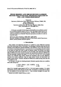
V. SIMULATION EXAMPLE: CAR CONTROL Consider a simple kinematic model of car control x& = v cos j, y& = v sin j, j& = v/l tan q, q& = u, where x and y are Cartesian coordinates of the rear-axle middle point, j is the orientation angle, v is the longitudinal velocity, l is the length between the two axles and q is the steering angle (Fig. 1). The task is to steer the car from a given initial position to the trajectory y = g(x), while g(x) and y are assumed to be measured in real time.

r

and r

(r-1)/r

r-1

|s| £ g0mtm , | s& | £ g1m

(r-1)

tm , ..., |s

1/r

| £ gr - 1 m tm

r

with e £ mtm . The parameter m roughly defines the regions, where one of the parameters e or tm is negligible. Consider a sampling law with the bounded variable sampling interval ì tM , ï ˆ ti+1 - ti = ti = íl | si |1 / r , ï tm , î

1/ r

l | sˆ i |

> tM ˆ t m < l | si |1 / r £ t M . l | sˆ i |1 / r £ t m

(15)

|s| £ r0e0, | s& | £ r1 e0

(r-1)

, ..., |s

| £ rr - 1 e0

1/r

2/3 -1/2

(r-1)

1/r

2/3

( s& + |s| sign s ) ] / 2/3 1/2 && |+ 2 (| s& |+ |s| ) ] [| s

can be applied here with a = 1. Substituting estimations z0, z1, && respectively, obtain z2 of s, s& , s 2/3 -1/2

u = - [z2+ 2 (|z1|+ | z0| )

2/3

(z1+ | z0| sign z0 )] / 2/3 1/2 [|z2|+ 2 (|z1|+ | z0| ) ]. (16)

Consider two possibilities: 6

3

z0 = sit , z1 = (si - si-1)t , z2 = si - 2si-1 + si-2,

.

With sufficiently small e and tm the asymptotics of Theorem 5 is established: (r-1)/r

Let v = const = 10 m/s, l = 5 m, g(x) = 10 sin(0.05x) + 5, x = y = j = q = 0 at t = 0. Define s = y - g(x). The relative degree of the system is 3 and the 3-sliding homogeneous quasicontinuous controller [23] && + 2 (| s& |+ |s| ) u = - a [s

Theorem 6. Let s be measured with sampling interval (15) and a noise of the magnitude e £ e0, the maximal measurement 1/r step being chosen in the form tM = max(be0 , tm), b > 0. Then for any sufficiently small l > 0 there are such positive constants m, g0, g1, ..., gr-1, r0, r1, ..., rr-1 that for any e0 ³ 0 controller (13) (or (14) with r = 3), (15) provides in finite time for keeping the inequalities (r-1)/r

Fig. 1. Kinematic car model

r

|s| £ g0e, | s& | £ g1 e , ..., |s | £ gr - 1 e with e > mtm , r (r-1)/r r-1 (r-1) 1/r r |s| £ g0mtm , | s& |£g1m tm , ..., |s | £ gr-1m tm with e£mtm . As follows from the Theorem, sampling step (15) features asymptotic properties of the constant step law and of (12) as

(17)

with a constant measurement step t (form (9)) and z0= si, z1=

si - si -1 s - si -1 si -1 - si - 2 , z2= ( i )/ti ti ti ti -1 -4

(18)

with the variable step (12), l = 0.15 and tm = 10 (form (14)). The control was applied only from t = 0.5 providing some time for the calculation of the finite differences. The

IEEE-TAC paper 05-383 integration was carried out according to the Euler method (the only one reliable with discontinuous dynamics) with the -5 integration step 10 on the time interval of 20 seconds in the absence of noises and on the time interval of 30 seconds otherwise. The tracking accuracy was calculated as maximal && | during the last 25% of the absolute values of |s|, | s& |, | s simulation time. The results are summarized in Table 1. -4 The system performance with t = 10 in the absence of noises is shown in Fig. 2. It cannot be distinguished from the performance with full exact measurements of all derivatives [23]. The system is fully destroyed already with the noise magnitude e = 0.0001 m. The system performance with the noise magnitude 0.1 m is practically the same as in the absence of noises with t = 0.2 s (Fig. 3). Note that the magnitude of the actual control q is about 16° and the vibration frequency is -1 about 0.5s , which is quite feasible. Mark that t = 0.2 s is close to the typical human reaction time. Note also that the real performance might be measured by the maximal steady-state distance of the car trajectory from the desired one, which is much smaller than sup|s| (Fig. 3a). Performance with the variable measurement step in the -4 absence of noises with l = 0.15 and tm = 10 is shown in Fig. 4. The accuracy |s| £ 4.0 is obtained with e = 0.05 (Fig. 5a, b). The performance of the controller is slightly improved by the restriction (15) of the measurement step from above. With large noises the restriction t £ tM = 0.2 actually provides for the same performance of the controller as with the constant sampling interval t = 0.2 (Fig. 5c,d). The demonstrated performance of the controllers does not significantly change when the noise frequency varies in the range from 10 to 100000. Table 1. Summary of the simulation results

6

-4

Fig. 2. Constant sampling step t = 10 , noise magnitude e = 0

Fig. 3. Constant sampling step t = 0.2s , noise magnitude e = 0.1m

Fig. 4. Variable measurement interval, noise magnitude e = 0 The simulation data listed in Table 1 confirm the asymptotics claimed in Theorems 3 - 6. It is seen that both variable-sampling-interval methods (16), (18), (12) and (16), (18), (15) provide for the ideal performance in the absence of noises, which does not differ from the results obtained with the

IEEE-TAC paper 05-383 sampling step fixed at the minimal step value. The constant step method (16), (17) actually identically performs with all noise magnitudes not exceeding some sensitivity threshold. After the noise exceeds the threshold the performance deteriorates. Variable sampling step provides for good performance in a large range of noise magnitudes, while the version with the sampling interval bounded from above looks preferable, if the maximal step is chosen sufficiently large.

VI. CONCLUSIONS High-order finite differences are shown to provide for robust output-feedback control when applied with homogeneous sliding-mode controllers. While the on-line robust differentiation is still the preferable way [20, 22, 23], the finite differences are to be considered as a real alternative in the case, when the sampling rate is too low to provide for the good differentiation accuracy. For example, simple calculation based on the simulation results and the asymptotic accuracy from [23] shows that in the absence of noises, in the considered simulation example, a second-order differentiator [20] in the feedback would provide for the accuracy of about |s| £ 6 with the sampling interval t = 0.02. That is much worse than the above-obtained performance with the constant measurement interval t = 0.2, when the finite differences are used. Due to the demonstrated robustness properties of the approach, it remains competitive, or may turn out to be even the only choice, when only low sampling rates are available. In particular, high-gain observer feedback implementation is impossible with the considered low sampling rates.

7

which provides for acceptable performance in the absence of noises, for the performance is not sensitive to small enough noises. The other way is to apply the variable measurement step control with unbounded ((11), (12)) or bounded ((12), (13)) step. In that case an excellent accuracy is provided with infinitesimally small measurement noises, and the controller is still robust. The best performance seems to be obtained with the bounded variable step (13), if some reasonable estimation of the maximal noise magnitude is available, and the maximal step is appropriately chosen. Thus, any strictly r-sliding-homogeneous finite-time-stable controller provides for the full SISO control based on the input measurements only, when the only information on the controlled uncertain process is actually its relative degree. The proposed technique is globally applicable if the relative degree is constant and few boundedness restrictions hold globally; it is also locally applicable to general-case weakly-minimumphase SISO systems. In the absence of noises the variablemeasurement-step strategy provides for the proportionality of r the resulting accuracy to tm , tm being the minimal sampling period and r being the relative degree. That is the best possible asymptotics with discrete sampling and discontinuous control [17]. In the presence of noises the tracking accuracy is proportional to the unknown noise magnitude. Only boundedness of the measurement noise is needed, no frequency considerations are relevant.

APPENDIX Proof of Theorem 3. Identity (8) implies equivalence of (9) and (11). It is known [6] that j-k

(k)

|D si /t

j-k

(j)

(j+1)

- s | £ (j - k) t sup|s

|, j = k + 1, ..., r - 1,

(j+1)

where sup|s | is calculated over the time interval containing (r) the involved sampling points. Recall that s is bounded. Denote (j+1)

ej(W) = (j - k) t supSÎW |s

|,

j = k + 1, ..., r - 1; j-k

Fig. 5. Variable measurement step with noise magnitude e = 0.05m; a, b: unbounded t; c,d: tM = 0.2 Finite differences can be implemented in two ways. In the case when the maximal measurement noise magnitude is known, the best way is to take a sufficiently large constant sampling interval providing for the best performance. If the noise magnitude cannot be estimated from above, a reasonable and the simplest way is still to choose the largest interval,

(k)

j-k

(j)

ej(W) = 0, j = 1, ..., k. Consider the difference D si /t - s as some noise of the magnitude ej which is infinitesimally small within any bounded area W when t ® 0. As follows from Theorem 2, with some small t0 all trajectories starting from some disk D centered at 0 concentrate in its subset W = r (r-1) {S Î R | |s| £ a0, | s& | £ a1, ..., | s | £ ar-1} to stay there forever. Apply transformation (t, S, e) a ( kt, dkS, dke) with such k > 1 that dkW Ì D. Since the transformation transfers trajectories into trajectories, achieve that with the enlarged r-j noise magnitudes ~e j = k ej the trajectories starting from dkD enter dkW Ì D in finite time to stay there. Taking into account r-j r-j that ~e j = 0 with j £ k and ~e j = k ej(D) = k t (j - k) (j+1)

supSÎD |s | = k ej(dkD) > ej(dkD) otherwise, achieve that the solutions of (4), (9) also enter dkW Ì D to stay there. Thus, s building infinite number of embedded sets dk D, s Î N, achieve the global finite-time convergence to the set W. It is easy to see that the transformation

IEEE-TAC paper 05-383 ~ Gk : (t, t, S)

a ( kt, k t, dkS)

preserves the discrete sampling and transfers the solutions of (4), (9) into the solutions of the same inclusion, but with a (r-1) different t. Let the set |s| £ a0, | s& | £ a1, ..., | s | £ ar-1 be attracting invariant set with some fixed sampling step t0. ~ Applying now Gk with k = t/t0 achieve the needed attractingset asymptotics.n Proof of Theorem 4. Denote by sˆ i( j ) the noisy measurement (j)

of s

j-k

i

, | sˆ i( j ) - si( j ) | £ bke

|D sˆ i( k ) /t

j-k

(j)

(r-j)/r

-(r-j)

= b kh

r-j

t , j = 1, ..., k. Then (j+1)

- s | £ ej(D) = (j - k)t supSÎW |s

r-j

| + Nj-kt ,

j = k + 1, ..., r - 1, Nj-k > 0. The rest of the proof is the same as of Theorem 3.n Proof of Theorem 5. The idea is to show by comparison with a suitable differential inclusion that the system has a global invariant attracting set. The needed asymptotics follows then immediately from the system homogeneity. With small e and 1/r tm the sampling step t » ls is close to zero near the plane s = 0, which means that the controller is highly sensitive to any noise. In order to remove the singularity enlarge the right-hand side of the inclusion (4), (5) taking | s |> 2e * , ì[-C , C ] + [ K m , K M ]j(S), s Îí î[-C - K M sup | j(S) |, C + K M sup | j(S) |], | s |£ 2e * . (r)

(19) Recall that j is globally bounded. Note also that even with e* = 0 solutions of (19) might be different from the solutions of (4), (5). As always, the inclusions are replaced here by the corresponding minimal Filippov differential inclusions. The idea is to show that solutions of (4), (12), (13) approximate solutions of (19), which in its turn approximate solutions of (4), (5). Controller (5) is finite-time stable, thus, the trajectories of the inclusion (4), (5) which start from a disk D0 centered at the origin terminate in finite time T in some smaller disk D1, being confined in some larger disk B during the time T . Call this the contraction property. Lemma 1. The contraction property of (4), (5) is preserved for (19) with somewhat enlarged D1, B, if e* > 0 is chosen small enough. Proof. Indeed, it follows from the Lagrange Theorem that the only possible limit point of the zeros of any solution s(t) of (r-1) (4), (5), or of (19), is the point where s = ... = s = 0, i.e. the origin S = 0. Therefore, the trajectories of (4), (5) and of (19) cross the hyperplane s = 0 not stopping on it. Hence, with e* = 0 the solutions of inclusion (19) are the same as of (4), (5). The Lemma follows now from the continuous dependence of the Filippov solutions on the right-hand side graph [8]. n Lemma 2. With l, e, tm small enough and |s| ³ 2 e* the i difference operators d , i = 1, 2, ..., r -1, are based on sampling outside of the layer |s| £ e*. Proof. Taking into account the boundedness of | s& | in B, 1/r require that l max | s& |(3 e*) < e*/r. That means that the maximal increment of |s| with the sampling taken inside the

8

layer |s| £ 2 e* and the noise magnitude e < e*, is less than e*/r. Thus, more than r sampling steps are needed for any point outside of the layer |s| £ 2 e* to be reached from the layer |s| £ e*. n Lemma 3. Let e* be defined from Lemma 1. Then with sufficiently small l the contraction property holds for (4), (12), (13) with somewhat enlarged D1, B and e, tm small enough. Proof. Show that outside of the layer |s| £ 2 e* controller (12), (13) can be considered as (5) with small measurement noises, which means that (12), (13) approximates (19) in the whole region. Let l be smaller than the value required in Lemma 2 and let tm and e be so small with respect to e* that only the first line of (12) is actual outside of |s| ³ e* and the identity tk = 1/r l| sˆ k | holds. According to Lemma 2 each measurement point of a trajectory outside of the layer |s| £ 2 e* is preceded by at least r measurements outside of |s| £ e*. Thus, with sufficiently small fixed l and correspondingly smaller e and tm the involved sampling steps are separated from zero. When l is small enough the feedback (12), (13) can be considered as sampling S in B1 = B Ç {|s| ³ e*} for (19) with small measurement errors. Indeed, it follows from the mean s (s) value formula s! d si = s (x) holding for some x Î [ti, ti-s] that s

(s)

(s+1)

s! |d si - s (ti)| £ lr supSÎB |s

1/r

| × supSÎB |s+e| .

The resulting motion satisfies “noisy” (19) and is described by the inclusion | s |> 2e * , (r) ì[-C , C ] + [ K m , K M ]u , s Îí î[-C - K M sup | j(S) |, C + K M sup | j(S) |], | s |£ 2e* , (20) with u defined from (12), (13). Due to the continuous dependence of the solutions on the right-hand-side graph, enlarging D1, B in an appropriate way, obtain the contraction property for “noisy” (19), and therefore for (4), (12), (13). Usage of (14) is justified by the asymptotic equivalence of 2 2 d si = (d sˆ i - d sˆ i -1 )/(ti + ti-1).and (d sˆ i - d sˆ i -1 )/ti with small l. n Let now e* = e*1 and l be fixed so that Lemmas 1-3 hold for sufficiently small e and tm. Lemma 4. There are a compact set W including the origin, and positive constants tm1 and e1, such that W is a global finite-time-attracting invariant set for (4), (12), (13) with any e £ e1 and tm £ tm1. Proof. Fix some values e and tm for which Lemma 3 holds. Let also tm and e be small enough with respect to e*1, so that the 1/r identity tk = l|sk| holds outside of |s| ³ e*1. Apply the transformation (t, tm, e, S)

r

a (kt, ktm, k e, dkS)

(21)

with k > 1. It preserves the trajectories of (4), (12), (13), which implies the contraction property with the set triplet dkB É dkD0 É dkD1

IEEE-TAC paper 05-383 for (4), (12), (13), and e and tm changed to the enlarged values r k e and ktm. Inside dkB these trajectories satisfy (12), (13), r (20) with correspondingly changed e* = k e*1, also (12), (13), (20) featuring the same contraction property (note that the restriction on l from the Lemma 2 proof is invariant with respect to transformation (21)). According to the above choice of tm its reduction does not influence trajectories of (12), (13), (20), therefore the reduction of ktm back to tm does not violate the contraction property of (4), (12), (13) with the sets dkD0, dkD1, dkB. In its r turn the reduction of k e back to e means just restriction to a subset of trajectories of (4), (12), (13) with smaller noises. Thus (4), (12), (13) with the original values of e and tm features the contraction property with the sets dkD0, dkD1, dkB for any k > 1. The same reasoning implies that the property is robust with respect to any reduction of e and tm. Choosing now k > 1 so that dkD1 still lies in the interior of D0 obtain that trajectories of (4), (12), (13) which start in l+1 l l+1 dk D0 terminate in dk D0 in the time k T without leaving l+1 dk B, l = 0, 1, .... Covering the whole space with the sets l dk D0, obtain the global finite-time convergence of the trajectories to the set D0. The point set of all trajectory segments starting in D0 and having the time-length T constitute the global attracting invariant set. n r Apply Lemma 4. Define m > 0 from the equality e1 = mtm1 . r Consider first the case when mtm £ e. Then applying 1/r transformation (21) with k = (e1/e) obtain (4), (12), (13) with e = e1, tm £ tm1 and the invariant set W. Now applying the inverse transformation and calculating the bounds of the attracting invariant set dkW obtain the needed asymptotics. Let r now mtm > e. Applying transformation (21) with k = tm1/tm obtain (4), (12), (13) with e < e1 and tm = tm1. After the inverse transformation obtain the other needed asymptotics, which ends the proof of Theorem 5. n Proof of Theorem 6. Choose some fixed sufficiently small value of l as in the proof of Theorem 5. Similarly to the previous proof obtain the contraction property and global invariant set attracting in finite time with any sufficiently small tm, e0, e = e0. Taking into account that (4), (13), (15) with the proposed in the Theorem choice of tM is invariant with respect to the transformation (t, tm, e0, S)

r

a ( k t, k tm, k e0, dkS)

readily obtain the first needed asymptotics. Consider now a compact region D0, including the origin and invariant with respect to (4), (5), such that all trajectories starting in it enter in finite time a smaller invariant compact subregion D1. Consider the “noisy” control ìï __ ( r -1) + [-d, d]), | s |> 2e * , u Î íco j(s + [-d, d], s& + [-d, d],..., s ïî[- sup | j(S) |, sup | j(S)], | s |£ 2e * , (22) __

where co denotes the convex closure operation, meaning here that the minimal segment is taken containing all the set. With sufficiently small d the above contraction property is preserved

9

for (4) (22) with somewhat changed invariant regions D0, D1 due to the continuous dependence on the right-hand-side-graph [8]. With sufficiently small l, tm, and e control (13), (15) satisfies (22) in D0, which means that the contraction property is true also for (4), (13), (15). Apply now the transformation (t, tm, e0, e, e*, d, S)

r

r

r

r

a ( kt, ktm, k e0, k e*, k e, k d, dkS)

with k > 1. Similarly to the proof of Theorem 5 obtain the contraction property of (4), (22) with changed parameters for dkD0, dkD1. But also (13), (15) with unchanged parameters satisfies (22) with dkD0 , dkD1. The rest of the proof is the same as of Theorem 5. n

REFERENCES [1] [2] [3] [4] [5] [6] [7] [8] [9] [10] [11] [12] [13] [14] [15] [16] [17] [18] [19] [20]

A. Bacciotti, L. Rosier, Liapunov functions and stability in control theory. Lecture notes in control and inf. sc. 267, Springer Verlag, London, 2001. G. Bartolini, A. Ferrara, E. Usai, “Chattering avoidance by second-order sliding mode control”, IEEE Trans. Automat. Control, vol. 43, no. 2, pp. 241-246, 1998. G. Bartolini, A. Pisano, E. Usai, “First and second derivative estimation by sliding mode technique”. Journal of Signal Processing, vol. 4, no. 2, pp. 167-176, 2000. G. Bartolini, A. Pisano, E. Punta, and E. Usai, “A survey of applications of second-order sliding mode control to mechanical systems”, International Journal of Control, vol. 76, no. 9/10, pp. 875-892, 2003. I. Boiko, L. Fridman, “Analysis of chattering in continuous slidingmode controllers”, IEEE Trans. Automat. Control, vol. 50, no. 9, pp. 1442- 1446, 2005. R. L. Burden & J. D. Faires; Numerical Analysis (seventh edition), Brooks/Cole, 1997. C. Edwards, S. K. Spurgeon. Sliding Mode Control: Theory and Applications, Taylor & Francis, 1998. A.F. Filippov. Differential Equations with Discontinuous Right-Hand Side, Kluwer, Dordrecht, the Netherlands, 1988. T. Floquet, J.-P. Barbot, and W. Perruquetti, "Second order sliding mode control for induction motor", in Proc. IEEE Conf. on Decision and Control, Sydney, Australia, 2000. T. Floquet, J.-P. Barbot, and W. Perruquetti, “Higher-order sliding mode stabilization for a class of nonholonomic perturbed systems”, Automatica, vol. 39, pp. 1077 –1083, 2003. L. Fridman, “Singularly perturbed analysis of chattering in relay control systems”, IEEE Trans. on Automatic Control, vol. 47, no.12, pp. 20792084, 2002. L. Fridman, “Chattering analysis in sliding mode systems with inertial sensors”, International Journal of Control, vol. 76, no. 9/10, pp. 906912, 2003. K. Furuta, Y. Pan, “Variable structure control with sliding sector”. Automatica, vol. 36, pp. 211-228, 2000. A. Isidori. Nonlinear Control Systems, second edition, Springer, New York, 1989. M.K. Khan, K.B. Goh, S.K. Spurgeon, “Second order sliding mode control of a diesel engine”, Asian J. Control, vol. 5, no. 4, pp. 614-619, 2003. S. Kobayashi, S. Suzuki, K. Furuta, “Adaptive VS differentiator”, Advances in Variable Structure Systems, Proc. of the 7th VSS Workshop, July 2002, Sarajevo. A. Levant (L.V. Levantovsky), “Sliding order and sliding accuracy in sliding mode control”, International Journal of Control, vol. 58, no. 6, pp.1247-1263, 1993. A. Levant. “Robust exact differentiation via sliding mode technique”, Automatica, vol. 34, no. 3, pp. 379-384, 1998. A. Levant. “Variable measurement step in 2-sliding control”. Kibernetica, vol. 36, no. 1, pp. 77-93, 2000. A. Levant, “Higher-order sliding modes, differentiation and outputfeedback control”, International J. of Control, vol. 76, no. 9/10, pp. 924-941, 2003.

IEEE-TAC paper 05-383 [21] A. Levant, “Finite Differences in Homogeneous Discontinuous Control”, in Proc. of the 44th IEEE Conference on Decision and Control, December 14-17, Atlantis, Paradise Island, Bahamas, 2004. [22] A. Levant, “Homogeneity approach to high-order sliding mode design”, Automatica, vol. 41, no. 5, pp. 823-830, 2005. [23] A. Levant, “Quasi-continuous high-order sliding-mode controllers”, IEEE Transactions on Automatic Control, vol. 50, no. 11, pp. 18121816, 2005. [24] A. Levant, A. Pridor, R. Gitizadeh, I. Yaesh, and J. Z. Ben-Asher, “Aircraft pitch control via second-order sliding technique”, AIAA Journal of Guidance, Control and Dynamics, vol. 23, no. 4, pp. 586594, 2000. [25] Z. Man, A.P. Paplinski, H.R. Wu, “A robust MIMO terminal sliding mode control for rigid robotic manipulators”, IEEE Trans. Automat. Control, vol. 39, no. 12, pp. 2464-2468, 1994. [26] Y. Orlov, “Finite time stability and robust control synthesis of uncertain switched systems”, SIAM J. Cont. Optim., vol. 43, no 4, pp. 1253-1271, 2005. [27] H. Sira-Ramírez, “On the dynamical sliding mode control of nonlinear systems”, International Journal of Control, vol. 57, no. 5, pp. 10391061, 1993. [28] H. Sira-Ramírez, “Dynamic Second-Order Sliding Mode Control of the Hovercraft Vessel”, IEEE Transactions On Control Systems Technology, vol. 10, no. 6, pp. 860-865, 2002. [29] I.A. Shkolnikov, Y.B. Shtessel, D. Lianos, & A.T. Thies, “Robust missile autopilot design via high-order sliding mode control”, in Proc. of AIAA Guidance, Navigation, and Control Conference, Denver, CO, AIAA paper No. 2000-3968, 2000. [30] Y.B. Shtessel, I.A. Shkolnikov, “Aeronautical and space vehicle control in dynamic sliding manifolds”, International Journal of Control, vol. 76, no. 9/10, 1000 - 1017, 2003. [31] Y.B. Shtessel, I.A. Shkolnikov, M.D.J. Brown, “An asymptotic secondorder smooth sliding mode control”, Asian J. of Control, vol. 5, no. 4, pp. 498-504, special issue on Sliding-Mode Control, 2003. [32] V.I. Utkin, Sliding Modes in Optimization and Control Problems, Springer, New York, 1992.

Arie Levant (formerly L. V. Levantovsky) received his MS degree in Differential Equations from the Moscow State University, USSR, in 1980, and his Ph.D. degree in Control Theory from the Institute for System Studies (ISI) of the USSR Academy of Sciences (Moscow) in 1987. From 1980 until 1989 he was with ISI (Moscow). In 1990-1992 he was with the Mechanical Engineering and Mathematical Depts. of the Ben-Gurion University (BeerSheva, Israel). From 1993 until 2001 he was a Senior Analyst at the Institute for Industrial Mathematics (Beer-Sheva, Israel). Since 2001 he is a Senior Lecturer at the Applied Mathematics Dept. of the Tel-Aviv University (Israel). His professional activities have been concentrated in nonlinear control theory, stability theory, singularity theory of differentiable mappings, image processing and numerous practical research projects in these and other fields. His current research interests are in high-order sliding-modes and their applications to control and observation, real-time robust exact differentiation and non-linear robust output-feedback control.

10