International Business & Economics Research Journal – January 2007
Volume 6, Number 1
Monte Carlo Simulation Of The Portfolio-Balance Model Of Exchange Rates: Finite Sample Properties Of The GMM Estimator Hong-Ghi Min, (Email:
[email protected]), Information and Communications University, Republic of Korea
ABSTRACT Using Monte Carlo simulation of the Portfolio-balance model of the exchange rates, we report finite sample properties of the GMM estimator for testing over-identifying restrictions in the simultaneous equations model. F-form of Sargan’s statistic performs better than its chi-squared form while Hansen’s GMM statistic has the smallest bias. INTRODUCTION
C
onsistent estimation of linear simultaneous equations model requires minimal set of identifying restrictions in the system and validity of those restrictions can be tested if a model is over-identified. While some statistics are developed and those statistics are widely applied to test the specification of the estimated equations, test the validity of the instrumental variables, and to test if the estimated equations encompass the reduced form little is known the small sample properties of those statistics. For this reason, We investigate the small sample properties of four different over-identifying test statistics for simultaneous equations model including Hausmann(1990)’s Likelihood-ratio test, Sargan(1958, 1960)’s minimum characteristic root statistic, Sargan(1980)’s corresponding F-statistic (Sargan, 1980), and Hansen(1982)’s GMM statistic. RESPONSE SURFACE METHODOLOGY, TEST STATISTICS, AND THE DGP Response Surface Methodology To overcome the specificity of Monte Carlo studies to the particular parameter and sample sizes employed, we utilize response surface methodology of Hendrey (1984). Let T be the finite sample probability of the test statistic lying in the critical region. In an experiment the DGP generates N sets of replications and the statistics lie in the critical region S out of N times. An explicit relationship can be defined as equation (7) in section 2.3. E(s) = πT = f (θ, T)
(1)
Monte Carlo estimator s gives: E(s) = πT = f (θ, T) + ε, εi ~ D(0, πT [1- πT]/N)
(2)
Let a is the analytically calculable asymptotic power of the test and p ( , T ) is the discrepancy between the finite sample and asymptotic power, i.e., T { p ( , T ) q ( , T )} .
1 / 2
1 / 2
1 / 2
Then,
p ( , T ) T
1/ 2
p( , T
1/ 2
)
(3)
holds. 63
International Business & Economics Research Journal – January 2007
Volume 6, Number 1
and the elements of . p ( , T ) is O (T ) and is a polynomial in powers of T Using (1)-(3), we can set up a stochastic relationship between a feasible and unbiased estimator of T and the unknown quantity a , , T as equation (4).
1/ 2
s a T
1/ 2
0
q( , T
1/ 2
1 / 2
)e
(4)
where q ( , T ) is an approximation to p( , T ) and the error e is the combination of and 1/ 2 1/ 2 1/ 2 1/ 2 1/ 2 T { p( , T ) q( , T )} . The choice of q ( , T ) is arbitrary but a finite polynomial in and T is 1/ 2 common and coefficients on the terms of q ( , T ) may be estimated by least squares. 1/ 2
1/ 2
The Test Statistics And Their Asymptotic Properties We consider four statistics whose statistical descriptions are given in Table 1. Table 1: Statistics Of Over-Identifying Restrictions Statistics Asymptotic Distributions (Degrees of freedom) Name Type Sources C0 IV Sargan (1958) Chi-squared (n) F0 IV Sargan (1980) Chi-squared with (m-k0) G0 GMM Hansen (1983) F(m- k0,T-m) L0 Likelihood- ratio test Harvey (1990) Chi-squared(n) (1). T is the econometric sample size, m is the number of instrumental variables, and ki is the number of coefficients estimated under Hi . (2). The statistic F0 is [C0/ (m-k0)]*[(T-m)/(T- k0)]/[1- C0/(T- k0)] which is C0/ (m-k0 ) plus finite sample adjustment arising from the finite sample boundedness of C0. (3). n is the number of over-identifying restrictions in the system.
The Data Generating Process: Portfolio-Balance Model Of Exchange Rates True reduced form [equations (7)-(8)] is derived from the true structural form [equation (5)-(6)]. For alternative structural form, x2,t 1 and x7,t 1 are falsely included into the system [equations (9)-(10)]. yt = α1Yt + β1 (y 2, t – x 7, t) + γ1Xt + ε 1, t, (ε 1, t:ε 2, t)’ ~ NID (O, Σ)
(5)
Yt = α2 + δy 1, t + γ2 Xt + ε 2, t
(6)
X t are 2 1 and 7 1 vectors of endogenous and exogenous variables at time t (t=1,….,T); X t ' ( x1t , x2t ,x3t ,x4t , x5t , x6t , x7t ) ; and are simultaneity parameters.
where ( yt , Yt )’ and yt 3
3 Xt
1 t ,
Yt 4
( 1t : 2t ) '
4 Xt
(7)
2t
(8)
Alternative structural model is given as equations (9) and (10). yt = α5 + β1 (y 2, t – x 7, t-1) + β2 (x 2, t – x 2, t-1) + γ5 Xt + ε 1, t, (ε 1, t : ε 2, t)’ ~ NID (0, Σ)
(9)
Yt = α6 + δy 1, t + γ6 Xt + ε 2, t
(10)
64
International Business & Economics Research Journal – January 2007
Volume 6, Number 1
Independent samples of endogenous variables are generated by the population defined in equation (5)-(10) a la Basmann (1960). Error terms are generated from linear transformation of i -N(0,1) and coefficients of transformation are from the Choleski decomposition of the variance-covariance matrices. The fraction of rejections s (=S/1,000) is an unbiased Monte Carlo estimator of the unknown finite sample rejection frequency T . EXPERIMENTAL DESIGN AND COMPUTATIONAL ASPECTS The Monte Carlo design variables for the econometric model (7)-(9) are and
( , , W , T ) { 0; 0}
T , where, (11)
and W = / , is the variance-covariance matrix of the reduced form equations and is the variancecovariance matrix of the structural form equations.
T [Ta , Tb ]
(12)
where Ta and Tb are the smallest and largest econometric sample size considered. For a given statistic (say) and critical value , the objective of Monte Carlo study is to find statistics’ finite sample rejection frequency T prob( ) for the DGP and those relationships of interest over .
T prob( , T ) g ( , T )
(13)
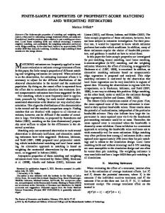
The value of key parameters 1 , , W , T cover a range typical of econometric models estimated with actual data: 1 =(0.3,0.8), 2 =2.244, =(0.4,0.7), T=(20,40,60,80), W =(0.4,0.6,0.8,0.9). All other parameters are from reported values of Branson et al (1979). The number of replications is 1,000. Given the choice of parameters, a full factorial design is adopted, resulting in 64 experiments in all. Structural model is estimated by two-stage least squares and Ordinary least squares are used for the reduced form. The asymptotic powers of four statistics were calculated with critical values corresponding to the 5 percent. POST-SIMULATION ANALYSIS This section approximates the finite sample properties of the test statistics by various analytical and numerical-analytical formulae, and examines how well these formulae perform. Response surface regressions are reported in Table 2. Nominal Size Of Four Statistics Response surface of nominal size is reported in the first panel of the Table 2. Most of the estimated coefficients are significant but that of S0. Size is well approximated for G0 while S0 is poorly approximated by the sample size and the ratio of the determinants. Using a conservative estimate of 0.016 for the standard deviation of sample proportions, we find that most estimators are significantly larger than the nominal size of 0.05. Most strikingly, L 0 mostly reject true null hypothesis implying that we need to a small sample adjustment for L0. Sargan (1980)’s Chi-squared test (S0) is biased and overreject in most of the cases in finite sample except for the case when simultaneity parameters are =0.8, =0.4, and T=80. F-form of Sargan’s statistic (F0) is less biased than S0 but properties of F0 resemble those of S0 as sample size increases. Hansen’s GMM statistic (G0) is also biased but nominal size of G0 approaches to the value of 0.05 while S0 departs significantly from 0.05. G0 has the least bias for the nominal size. Asymptotic Power Of Four Statistics Figure 1 shows that, for most of the cases, estimated nominal power decreases as the econometric sample size increases and it increases with the increase of w. Asymptotic power is best approximated for G0 and then F0 while S0 is poorly approximated. 65
International Business & Economics Research Journal – January 2007
Volume 6, Number 1
Table 2: Response Surface Regressions PANEL A
Constant T W
Adj R2 PANEL B
Constant T W
Adj R2 PANEL C
G0 2.5151(0.2439)** -0.0324(0.0032)** 0.9434(0.1802)** -57.991(6.085)** 0.607
Nominal Size of S0 1.9174(0.3184)** -0.0203(0.0043)** 0.6384(0.2444)** -36.458(7.942)** 0.261
F0 1.7900(0.3278)** -0.0186(0.0044)** 0.8187(0.2516)** -46.874(8.177)** 0.405
G0 2.1533(0.2025)** -0.0270(0.0027)** 0.7237(0.1496)** -45.537(5.052)** 0.6082
Asymptotic Power of S0 1.5877(0.3051)** -0.1363(0.0041)** 0.4901(0.2341)* -28.064(7.61)** 0.1627
F0 1.8591(0.3032)** -0.0173(0.0041)** 0.8497(0.2327)** -48.597(7.563)** 0.5082
Finite Sample Power of L0 G0 S0 Constant 0.0603(0.3088) -0.4286(0.1573)* -0.1383(0.207) T 0.0040(0.0100) 0.0085(0.0021)** 0.0027(0.0029) W 0.0100(0.2281) -0.1859(0.1162) 0.0663(0.1596) -1.5383(7.704) 12.401(3.924)** 1.6375(5.2384) Adj R2 0.0856 0.2041 0.0101 Note: Double asterisks denote significance at 1 % critical level and single asterisk for 5%.
F0 0.1934(0.1711) 0.0193(0.0023)** -0.0444(0.1330) 1.9975(4.1438) -0.0623
L0 has rejection probability of one in most of the cases and S0 appears to be more powerful than F0 and G0 unless simultaneity parameter is large. Another interesting feature is that S 0 outperform F0 even in small samples but G0 has the smallest rejection probability. Finite Sample Power Of Four Statistics In order to compare tests in terms of their power of a given size, the critical value for each test is set with reference to the empirical distribution of the statistic corresponding to the empirical size of 0.05. In each replication, the false null is rejected if the test statistic exceeded the empirical critical value. Most of the estimates for the response surface regressions reported in Table 2 are insignificant and they poorly approximate the finite sample power of these statistics. However, for G0, the estimated coefficient of T is significant and finite sample power of G0 increases with the increase of T. For all statistics, empirical power increase with the increase of sample size and empirical power decrease with the increase of w for most of the cases. Out of four statistics, L0 is the most powerful test statistic in most of the cases and its finite sample power increase with the increase of the econometric sample size. G0 comes next and then F0 and S0. However, performance of F0 and S0 are quite similar. Estimated finite sample power is much smaller than its asymptotic power substantially. Most significant departure between asymptotic power and finite sample power comes for S 0 while G0 approximates its asymptotic power well. Finite sample power of L0 is larger than other statistics and this increases with the increase of econometric sample size.
66
International Business & Economics Research Journal – January 2007
Volume 6, Number 1
Figure 1: Finite Sample Properties Of L0, G0, S0, and F0 Asymtotic Size of Test Statistics 1.0
S0 G0 F0
Probability of Rejection
0.8
0.6
0.4
0.2
0.0 5
10
15
20
25
30
35
40
45
50
55
60
Finite Sample Power of Test Statistics 1.00
L0 S0 G0 F0
Probability of Rejection
0.75
0.50
0.25
0.00 5
10
15
20
25
30
35
40
45
50
55
60
55
60
Asymtotic Power of Test Statistics 1.0
S0 G0 F0
Probability of Rejection
0.8
0.6
0.4
0.2
0.0 5
10
15
20
25
30
35
67
40
45
50
International Business & Economics Research Journal – January 2007
Volume 6, Number 1
CONCLUSIONS We conducted a Monte Carlo experiment to investigate the small sample properties of the four statistics which test the over-identifying restrictions in the simultaneous equations model. The likelihood-ratio test tends to reject the null hypothesis even when the errors in the model are consistent with the statistic’s embodied hypothesis in the two equations model in finite sample. Small sample adjustment of Godfrey and Pesaran (1983) can be a solution for this bias. The problem seems less severe with test statistics of S 0, F0, and G0. The use of G0 helps a little but it is also biased in finite sample. F-form of Sargan’s statistic (F0 ) performs better than its Chi-squared form ( S0 ). Hansen’s GMM statistic (G0) has the smallest bias. Different methodology and software may allow more extensive design and more efficient simulation and control variate might help estimate T more efficiently. REFERENCES 1. 2. 3. 4. 5. 6. 7. 8. 9. 10.
Basmann, R. L., 1960, On Finite Sample Distributions of Generalized Classical linear identifiability Test Statistics, Journal of American Statistical Association, 55, 650-659. Branson, W. H., Halttunen, H., and Masson, P., 1979, Exchange Rates in the Short-run: Some Further Results, European Economic Review, 12, 395-402. Byron, R. P., 1974, Testing Structural Specifications Using the Unrestricted Reduced Form, Econometrica, 42, 869-883. Ericsson, N. R., 1991, Monte Carlo Methodology and the Finite Sample Properties of the Instrumental variables Statistic for Testing Nested and Non-nested Hypothesis, Econometrica, 42, 869-883. Godfrey, L. G. and Pesaran, M. H., 1983, Tests of Non-nested Regression Model: Small Sample Adjustment and Monte Carlo Evidence, Journal of Econometrics, 21, 133-154. Harvey, A., 1990, The Econometric Analyses of Time Series, London:Phillip Allan. Hansen, L. P., 1982, Large Sample Properties of Generalized Method of Moments Estimator, Econometrica, 50, 1029-1054. Hendrey, D. F., 1984, Monte Carlo Experimentation in Econometrics, Chapter 16 in Handbook of Econometrics, volume 2, ed. By Grilliches and Intrilligatot, M. D., Amsterdam: North-Holland. 937-976. Sargan, J. D., 1958, The Estimation of Economic Relationships Using Instrumental Variables, Econometrica, 26, 393-415. Sargan, J. D., 1980, Some Approximations to the Distribution of Econometric Criteria Which are Asymptotically Distributed as Chi-squared, Econometrica, 48, 1107-1138.
68