Journal of the Eastern Asia Society for Transportation Studies, Vol. 6, pp. 1667 - 1681, 2005
THE FINITE-SAMPLE PROPERTIES OF MAXIMUM LIKELIHOOD ESTIMATORS IN MULTINOMIAL PROBIT MODELS Yu-Chin CHEN Ph. D. Student Department of Transportation and Communication Management Science National Cheng Kung University 1, University Road, Tainan 70101, Taiwan, R.O.C. Fax: +886-6-2753882 E-mail:
[email protected]
Liang-Shyong DUANN Professor Department of Marketing and Logistics Southern Taiwan University of Technology 1, Nantai St., Yung-Kang, Tainan 71005, Taiwan, R.O.C. Fax: +886-6-2753882 E-mail:
[email protected]
Wan-Pei HU Ph. D. Student Department of Transportation and Communication Management Science National Cheng Kung University 1, University Road, Tainan 70101, Taiwan, R.O.C. Fax: +886-6-2753882 E-mail:
[email protected] Abstract: In this paper we discuss the finite-sample properties of maximum likelihood estimators of multinomial probit model. Sample sizes ranging from 20 to 200 at interval of 10 are tested. For each sample size, we estimated 9 utility specifications under different error covariance matrix assumptions. Robust variance matrix is used to get the asymptotic covariance of estimators for each model. We use Monte Carlo experiments to generate the data sets and replicate 500 times for each experiment. We found that when the size of standardized parameter of generic variable is greater than 0.5 and the sample size is greater than 60, the odds of getting significant estimator that is close to the true value are larger than 0.9. When the size of standardized parameter is small, e.g., less than 0.25, a sample size of at least 170 is needed to get good results. Key Words: probit, Type I error, Type II error, correlation, Monte Carlo simulation, robust variance matrix 1. INTRODUCTION The selection of discrete choice models is generally a tradeoff between functional flexibility and computational feasibility. On the one extreme is the computationally efficient but inflexible multinomial logit (MNL) model (McFadden, 1974). The estimation of MNL model is relatively easy due to its closed functional form and unique solution property. However, its independent of irrelevant alternatives (IIA) assumption limits its application when similarities among alternatives exist. Brundell-Freij (1997), Munizaga, Heydecker, and Ortúzar (1997), among others, have shown that ignoring correlations between alternatives may cause biased estimates. On the other extreme is the computationally inefficient but flexible multinomial probit (MNP) model (Daganzo, 1979). MNP model assumes error terms to be multivariate normally distributed and allows any error structure in theory. So it can specify correlations 1667
Journal of the Eastern Asia Society for Transportation Studies, Vol. 6, pp. 1667 - 1681, 2005
between alternatives and allows different variances among alternatives. In recent years, it has been used in many travel choice situations where similarities of alternatives may exist, e.g., Hausman and Wise (1978), Chintagunta (1992), Yai, et al (1997) and Bolduc (1999). The estimation of MNP model needs to evaluate multidimensional integrals, thus causes some computational barriers. The most common method of calibrating discrete choice models is maximum likelihood estimation (MLE). The asymptotical property of MLE means that the sample size is important both in estimation and inference (Shenton and Bowman, 1977). However, in many travel choice situations, researchers can only obtain limited samples due to time, cost, or population limitations. The calibration burden of MNP model sometimes also put constraints on its sample size. MLE method estimates only asymptotically efficient standard errors. What constitutes an adequate sample size to avoid the inference problem is not at all clear. This problem is often ignored or is regarded as of little significance. Eliason (1993) argued that for a model with only a few parameters to estimate, a sample size of more than 60 was usually large enough. However, to which sample size the standard error of MNP model begins to fail is basically unknown. With small sample size, the similarities among alternatives may cause unreliable estimators of standard error which statistical inference is based. To our knowledge, no research has deal with the finite-sample properties of MLE estimators in MNP models. The purpose of this paper is to investigate the extent of sampling bias in parameter estimates of MNP model and how this bias is affected by the degree of correlation between alternatives. This is carried out through the application of MNP estimation to many artificially generated data sets, with known values of the parameters. Hsiao (2002) showed that when error terms were correlated with dependent variables and nonlinear models were misspecified, then parameter estimates would generally be inconsistent. Guilkey and Murphy (1993) showed that misleading results would be obtained if Hessian matrix was used for hypothesis testing in random effects probit model. Newey and West (1987) argued that the so-called robust variance matrix would obtain valid asymptotic variance whether the model was correctly specified or not. In this paper we will test the performance of robust variance matrix for both correctly and incorrectly specified MNP models. This paper is organized as follows. In section 2, we briefly introduce MNP model. Section 3 discusses the utility functions, error structures, and data generating processes. Section 4 introduces the hypotheses tested, robust variance matrix, and estimation method. We present the simulation results in section 5. The test results of 9 different error structures for 19 different sample sizes are discussed. The effect of sample size on robust variance matrix is also discussed. Last section presents the summary of results and discussions. 2. MULTINOMIAL PROBIT (MNP) MODEL In a standard discrete choice situation, the indirect utility of an individual i (i=1,…,N) choosing alternative j (j=1,…,J) is given by U ij = β ′x ij + εij (1) where x ij is a vector of explanatory variables includes alternative j’s attributes and individual i’s social-economic characteristics. β is the associated vector of parameters and 1668
Journal of the Eastern Asia Society for Transportation Studies, Vol. 6, pp. 1667 - 1681, 2005
εij is the random error.
A typical representation of the probability that individual i selects alternative j is given by pij = Prob ⎡⎣U ij >U ik for all j ≠ k ⎤⎦
(2)
MNP model (Daganzo, 1979) is derived by the assumption that random error εij ’s are multivariate normally distributed: pij = ∫
εj ε1 =−∞
∫
εj εj −1 =−∞
∫
∞ εj =−∞
∫
εj εj +1 =−∞
∫
εj εJ =−∞
f (ε1 ,..., εJ |U , Σε )d ε1 ,
,d εJ
(3)
where f (i|U , Σε ) is the multivariate normal density function with mean U J ×1 and covariance matrix ΣJε×J . The error structure of MNP model allows correlation between alternatives. One can analyze the similarity pattern of alternatives by specifying the corresponding covariance structure ΣJε ×J . There are J(J+1)/2 unknown parameters in the J×J covariance structure. However, the identification condition requires that at most J(J-1)/2-1 covariance parameters can be estimated (Horowitz, 1991; Bunch, 1991). All model discussed in this paper are identified. The log-likelihood function for the observed samples is N J ln L = ∑ i =1 ∑ j =1yij ln pij (4) where yij = 1 , if individual i chooses alternative j ; and yij = 0 , otherwise.
3. EXPERIMENTAL DESIGN AND MONTE CARLO SIMULATION Our primary concern in this paper is to investigate the inferential problems when researchers utilize MLE in finite-samples. We examine this problem by the odds of Type I and Type II errors at various sample sizes. 500 data sets were generated for each sample sizes according to given utility function and parameters. MNP models were calibrated with these data sets. The estimated coefficients were tested against given parameters to decide the odds of Type I and Type II errors. 3.1 Utility function We specify the utility function of individual i in a three-alternative choice situation as: U 1i = α1 U 2 i = α2 U 3i =
−β1 ⋅ x1i −β1 ⋅ x 2i −β1 ⋅ x 3i
−β2 ⋅ z1i −β2 ⋅ z 2i −β2 ⋅ z 3i
+δ1 ⋅ ai +δ2 ⋅bi
+ε1i +ε2i +ε3i
(5) (6) (7)
The above “true” utility function includes three distinct types of variables (alternative specific dummies, generic variables, and alternative specific variables) that are generally used in travel demand models. The parameters of alternative specific dummies are α1 and α2 . They are generally called alternative specific constants. There are two generic variables x and z whose values are varied among individuals and alternatives. The parameters of generic variables ( β1 and β2 ) are indifferent among alternatives. The values of alternative specific variables a and b are determined by the socio-economic characteristics of individual i. Their parameters δ1 and δ2 are alternative-specific. This specification is similar to a three-mode
1669
Journal of the Eastern Asia Society for Transportation Studies, Vol. 6, pp. 1667 - 1681, 2005
(e.g., auto, bus, rail) choice situation in which travel time and travel cost are generic variables while auto ownership and number of transfers are alternative specific variables. 3.2 Data Set Generating 500 data sets for each experiment are generated. Each data set are generated by the following process. First, six parameters are given the following “true” values. α1 =-0.2, α2 =0.4, β1 =-0.25, β2 =-0.5, δ1 =0.3, and δ2 =0.6. Then, the values of x ’s, z ’s, a ’s and b ’s are generated from standardized normal distribution N(0,1) using pseudo-random number generator. We also generated the values of variables from a uniform distribution [−0.5,0.5] . The results are similar so we do not report them in this paper for brevity. Because the degree of similarity between alternatives may affect the estimates of parameters, we consider the following covariance matrices for the disturbance terms: (1). No Correlation:
(2). Correlation between Alternatives 1 and 2:
⎡1 ⎤ ⎢ ⎥ ΣA = ⎢0 1 ⎥ ⎢ ⎥ ⎢0 0 1⎥ ⎣ ⎦
⎡1 ⎤ ⎢ ⎥ ΣB = ⎢.25 1 ⎥ , ⎢ ⎥ ⎢ 0 0 1⎥ ⎣ ⎦
(3). Correlation between Alternatives 1 and 3: ⎡1 ⎤ ⎢ ⎥ ΣD = ⎢ 0 1 ⎥ , ⎢ ⎥ ⎢.25 0 1⎥ ⎣ ⎦
⎡1 ⎤ ⎢ ⎥ ΣE = ⎢ 0 1 ⎥ ⎢ ⎥ ⎢.75 0 1⎥ ⎣ ⎦
⎡1 ⎤ ⎢ ⎥ ΣC = ⎢.50 1 ⎥ ⎢ ⎥ ⎢ 0 0 1⎥ ⎣ ⎦
(4). Alternative 1 is equally-correlated with Alternative 2 and 3: ⎡1 ⎤ ⎢ ⎥ ΣF = ⎢.25 1 ⎥ , ⎢ ⎥ ⎢.25 0 1⎥ ⎣ ⎦
⎡1 ⎤ ⎢ ⎥ ΣG = ⎢.50 1 ⎥ ⎢ ⎥ ⎢.50 0 1⎥ ⎣ ⎦
(5). All alternatives are equally-correlated: ⎡1 ⎤ ⎢ ⎥ ⎢ ⎥ , ΣH = .25 1 ⎢ ⎥ ⎢.25 .25 1⎥ ⎣ ⎦
⎡1 ⎤ ⎢ ⎥ ⎢ ⎥ ΣI = .75 1 ⎢ ⎥ ⎢.75 .75 1⎥ ⎣ ⎦
For each trial of an experiment, three error terms (ε1 , ε2 , ε3 ) corresponding to a particular tri-variate normal covariance matrix are drawn using following equation: ε = Lη (8) ε (9) Σ = LL ′ where η is standard normal random number and L is defined as a lower-triangular matrix from Cholesky decomposition. After x ’s, z ’s, a ’s, b ’s, and ε ’s are drawn, U ji is constructed using equations (5)-(7)and given parameter vector (α1 , α2 , β1 , β2 , δ1 , δ2 ) . The y ji ’s are then calculated as follows: ⎧⎪1 if U ji ≥U j ′i for j ′ = 1,...,J , and y ji = ⎪⎨ ⎪⎪0 otherwise. ⎩
(10)
New samples of x is ’s, z is ’s, ai ’s and bi ’s are drawn according to the sample sizes. We repeat this process 500 times for each experiment in the same sample size. That is, we conduct 500 experiments for each sample size and covariance matrix combination. Since there are 9 covariance matrices, we carried out 4,500 (500×9) experiments for each sample size. 1670
Journal of the Eastern Asia Society for Transportation Studies, Vol. 6, pp. 1667 - 1681, 2005
Shenton and Bowman (1977) showed that there might be inference problems when sample size was less than 30. So we conduct this research for sample sizes ranging from 20 to 200 at intervals of 10 (i.e., n=20, 30… etc.). 4. TEST FOR SIGNIFICANCE Statistical theory and conventional experiences suggest that standard errors might be inefficient as sample size declines. This property has an important meaning for classical hypothesis testing. We examine it through the test of Type I error and Type II error. 4.1 Type I Error and Type II Error Type I error occurs when a true hypothesis is rejected. In practice, Type I error will occur when the ratio of an estimate to its standard error produces a test statistic large enough to permit the rejection of null hypothesis even though it is true. Type II error occurs when we fail to reject a false hypothesis. In practice, Type II error will occur when the ratio of an estimate to its standard error produces a test statistic too small to reject the null hypothesis even though it is false. In this paper, the true parameters of variables are given, so we use Eq.(11) to examine if Type I error occurs. We first calculate t-values according to Eq.(12) for parameters (α1 , α2 , β1 , β2 , δ1 , δ2 ) . Then we adopt significance level at 0.05 for the two-tail test, which is fairly standard for the discipline. If a t-value falls into the rejection area, we will reject null hypothesis. For given level of significance, the boundary of rejection area is set by the critical t-values which are determined by the degree of freedom. In each case of ours, the degree of freedom is the number of samples minus the number of parameters to be estimated. Since the null hypothesis is true, we will make a Type I error. Finally, we divide the number of Type I errors we made by the number of experiments (i.e., 500) in each sample size and covariance matrix combination to get the probability of Type I error for that combination. We called this probability Type I error rate. H 0 : β = βtrue , H1 : β ≠ βtrue t = βˆ − βtrue s .e. βˆ
(12)
Pr (Type I error ) = Pr (Reject H 0 | H 0 is true)
(13)
(
)
()
(11)
We use Eq.(14) and (15) to examine Type II error. Since the “true” values of parameters are given, we only test directional hypotheses. We also adopt significance level at 0.05. If a t-value does not fall into the rejection area, we will fail to reject the null hypothesis. Since the null hypothesis is not true, we will make a Type II error. The probability of making Type II error (Type II error rate) is calculated similar to Type I error rate. H 0 : β = 0, H1 : β > 0 or β < 0 t = βˆ − 0 s .e. βˆ
(14)
Pr (Type II error ) = Pr (Fail to Reject H 0 | H1 is true)
(16)
(
)
()
(15)
We use Eq.(11) and (12) to examine whether Type I error exists. This is the standard 1671
Journal of the Eastern Asia Society for Transportation Studies, Vol. 6, pp. 1667 - 1681, 2005
procedure in the statistical inference. When the calculated t-value falls outside the rejection area, we will fail to reject the null hypothesis and conclude that the estimated coefficient βˆ is insignificantly different from the true parameter β . However, when the standard error of βˆ is large, the calculated t-values in Eq.(12) may be small even when the difference between βˆ and β is quite large. This may cause the result of failing to reject null hypotheses in Eq.(11). The same situation will happen for Eq.(14) and (15). So we will get the conclusion that βˆ is insignificantly different from both β and 0. The results are contradictory. Since one result says that the corresponding variable of β has no effect on the dependent variable, i.e., β =0, while the other result says that the corresponding variable of β has significant effect on the dependent variable, i.e., β = βtrue ≠ 0 . To solve this problem, we define a statistic called Accuracy Rate (AR). If we fail to reject null hypothesis in Eq.(11) but reject the null hypothesis in Eq.(14), then we call the estimated coefficient “accurate”. The accuracy rate is defined as Eq.(17) and calculated similar to Type I error rate.
(
)
Accuracy Rate (AR ) = Pr βˆ = β , and β ≠ 0
(17)
4.2 Variance of the Estimates Eq. (18) stands for a correctly specified model (White, 1984). It says that the estimate βˆ converges to true parameter β * and (βˆ − β * ) is normally distributed as the sample size approaches infinity.
(
)
d
(
)
−1 n βˆ − β * → N 0,(−H ) ,
n →∞
N ⎛ ∂L2i ⎞⎟ ⎟⎟ H= ∑ ⎜⎜⎜ ⎟ i=1 ⎝ ∂β∂β ′ ⎠
(18) (19)
where β * is the true parameter vector, βˆ is the maximum likelihood estimator, L is log-likelihood function, and H is the Hessian matrix. White (1982) pointed out that if the model is not correctly specified, the variances of estimates calculated according to Eq.(18) may not be correct. Newey and West (1987) developed a robust variance matrix formula to encompass autocorrelated and heteroscedastic error terms. They defined the asymptotic covariance of βˆ as
(
)
d
n βˆ − β * → N (0, H -1VH -1 ) ,
n →∞
N ⎛ ∂L ⎞′ ⎛ ∂L ⎞ V = ∑ ⎜⎜ i ⎟⎟ ⎜⎜ i ⎟⎟ ⎜ ⎟⎜ ⎟ i =1 ⎝ ∂β ⎠ ⎝ ∂β ⎠
(20) (21)
where V is the variance of the scores. When the model is correctly specified, the matrix –H=V according to the information matrix equality principle, so H -1VH -1 = −H -1 (White, 1982). The variances of estimates calculated by Eq.(18) and Eq.(20) will be the same. However, if the model is not correctly specified, the score function is generally invalid, Hessian matrix is not robust, and the t-values are unreliable. The asymptotic variance of βˆ in Eq.(20) is so-called robust covariance matrix, since it is always valid whether the model is correctly specified or not.
1672
Journal of the Eastern Asia Society for Transportation Studies, Vol. 6, pp. 1667 - 1681, 2005
4.3 Estimation The estimation of MNP models can be achieved by the simulated maximum likelihood approach (Lerman and Manski, 1981) using the GHK simulator (Borsch-Supan and Hajivassiliou, 1993). Despite the development of advanced computer technology, the above approach is still very demanding of computing time (Munizaga, et al, 1997). In this paper, we use a numerical method provided by GAUSS package, Gauss-Legendre integration, to estimate MNP model. The main advantage of this approximately numerical approach is that the likelihood function can be easily and well calculated for any values of the parameters, especially when the dimension of integration is small. This approach is very suited for our study which has three alternatives and two dimensions of integration. 5. RESULTS AND DISCUSSIONS We conducted this research for 19 sample sizes ranging from 20 to 200 at an interval of 10. For each sample size, we estimated 9 models under different error covariance matrix assumptions. So the number of model specifications and sample size combinations is 171. For each model specification and sample size combination, we conducted 500 experiments and used their results to compute Type I error rate, Type II error rate, and accuracy rate (AR). The results for sample size n=50 and 150 are shown in Table 1 and Table 2. The complete results for model ΣA are shown in Figure 1. The comparison of models ΣA , ΣB , and ΣC for selected parameters are shown in Figure 2. The rest results are not reported here for brevity. We also discussed the results of correctly specified models and misspecified models in this section. 5.1. Correctly Specified models We separated nine models into different groups according to their covariance matrices in the following discussion. (1). No correlation model (model ΣA ) Type I error rates for parameters β1 and β2 are around 0.06 for sample size larger than 60. Type II error for parameter β2 is very low for sample size larger than 60. However, Type II error rate for parameter β1 is larger than 0.1 if the sample size is smaller than 150. The accuracy rate for parameter β2 is quite high (>0.9) for sample size larger than 60. But the same accuracy rate for parameter β1 can not be obtained unless the sample size is larger than 170. The results of Type I error rate for parameters α1 , α2 , δ1 , and δ2 are similar to those of β1 and β2 . They are around 0.06 when the sample size is larger than 60. However, Type II error rates are very high for parameters α1 and δ1 even when the sample size is 200. Type II error rates for parameters δ2 and α2 are quite low if the sample size is larger than 150. The results of accuracy rate is similar to those of Type II error rate. The accuracy rates for parameters α1 and δ1 are quite poor even when the sample size is 200. The accuracy rates for parameters δ2 and α2 are acceptable (>0.8) when the sample size is large than 170. The values of variables x , z , a and b are randomly drawn from standardized normal distribution N(0,1), so their parameters are standardized parameters. These parameters’ sizes 1673
Journal of the Eastern Asia Society for Transportation Studies, Vol. 6, pp. 1667 - 1681, 2005
Table 1. Comparison of Probit Models in Various Error Structures (Sample Size=50, Replication = 500) Abbreviated Error Structure ⎡σ21 σ22 ⎤ ⎢ ⎥ ⎢σ31 σ32 ⎥ ⎣ ⎦ β1 = −0.25
Type I Error Rate Type II Error Rate Accuracy Rate
Model ΣA
Model ΣB
Model ΣC
Model ΣD
Model ΣE
Model ΣF
Model ΣG
Model ΣH
Model ΣI
⎡0 1 ⎤ ⎢0 0⎥ ⎣ ⎦
⎡ .25 1⎤ ⎢ ⎥ ⎢ 0 0⎥ ⎣ ⎦
⎡ .50 1⎤ ⎢ ⎥ ⎢ 0 0⎥ ⎣ ⎦
⎡ 0 1⎤ ⎢ ⎥ ⎢ .25 0⎥ ⎣ ⎦
⎡ 0 1⎤ ⎢ ⎥ ⎢ .75 0⎥ ⎣ ⎦
⎡ .25 1⎤ ⎢ ⎥ ⎢ .25 0⎥ ⎣ ⎦
⎡ .50 1⎤ ⎢ ⎥ ⎢ .50 0⎥ ⎣ ⎦
⎡ .25 1 ⎤ ⎢ ⎥ ⎢ .25 .25⎥ ⎣ ⎦
⎡ .75 1 ⎤ ⎢ ⎥ ⎢ .75 .75⎥ ⎣ ⎦
0.074 0.512 0.434
0.128 0.494 0.442
0.110 0.458 0.486
0.098 0.488 0.462
0.080 0.366 0.590
0.112 0.526 0.432
0.082 0.420 0.534
0.020 0.712 0.280
0.052 0.516 0.464
0.086 0.050 0.886
0.130 0.108 0.788
0.094 0.068 0.854
0.084 0.102 0.844
0.078 0.038 0.888
0.126 0.140 0.754
0.108 0.078 0.818
0.016 0.454 0.540
0.010 0.446 0.544
0.050 0.792 0.162
0.166 0.794 0.056
0.100 0.850 0.060
0.056 0.824 0.144
0.084 0.754 0.196
0.154 0.882 0.030
0.108 0.898 0.040
0.064 0.872 0.096
0.056 0.856 0.128
0.070 0.578 0.380
0.086 0.648 0.298
0.054 0.656 0.312
0.09 0.662 0.274
0.056 0.568 0.388
0.088 0.598 0.344
0.062 0.568 0.394
0.060 0.774 0.216
0.030 0.618 0.378
0.092 0.704 0.230
0.092 0.750 0.190
0.064 0.702 0.260
0.098 0.784 0.168
0.104 0.616 0.338
0.052 0.744 0.226
0.066 0.654 0.302
0.046 0.874 0.114
0.024 0.720 0.274
0.086 0.336 0.604
0.074 0.356 0.604
0.068 0.336 0.628
0.090 0.396 0.554
0.084 0.324 0.624
0.080 0.388 0.560
0.084 0.314 0.628
0.028 0.680 0.318
0.012 0.474 0.520
N/A N/A N/A
0.398 0.552 0.050
0.334 0.494 0.174
0.402 0.522 0.076
0.33 0.286 0.384
0.306 0.614 0.080
0.338 0.448 0.214
0.044 0.914 0.076
0.236 0.258 0.510
β2 = −0.50
Type I Error Rate Type II Error Rate Accuracy Rate α1 = −0.2
Type I Error Rate Type II Error Rate Accuracy Rate α2 = 0.4
Type I Error Rate Type II Error Rate Accuracy Rate δ1 = 0.3
Type I Error Rate Type II Error Rate Accuracy Rate δ2 = 0.6
Type I Error Rate Type II Error Rate Accuracy Rate ρ = .25, .5, .75
Type I Error Rate Type II Error Rate Accuracy Rate
1674
Journal of the Eastern Asia Society for Transportation Studies, Vol. 6, pp. 1667 - 1681, 2005
Table 2. Comparison of Probit Models in Various Error Structures (Sample Size=150, Replication = 500) Abbreviated Error Structure ⎡σ21 σ22 ⎤ ⎢ ⎥ ⎢σ31 σ32 ⎥ ⎣ ⎦ β1 = −0.25
Type I Error Rate Type II Error Rate Accuracy Rate
Model ΣA
Model ΣB
Model ΣC
Model ΣD
Model ΣE
Model ΣF
Model ΣG
Model ΣH
Model ΣI
⎡0 1 ⎤ ⎢0 0⎥ ⎣ ⎦
⎡ .25 1⎤ ⎢ ⎥ ⎢ 0 0⎥ ⎣ ⎦
⎡ .50 1⎤ ⎢ ⎥ ⎢ 0 0⎥ ⎣ ⎦
⎡ 0 1⎤ ⎢ ⎥ ⎢ .25 0⎥ ⎣ ⎦
⎡ 0 1⎤ ⎢ ⎥ ⎢ .75 0⎥ ⎣ ⎦
⎡ .25 1⎤ ⎢ ⎥ ⎢ .25 0⎥ ⎣ ⎦
⎡ .50 1⎤ ⎢ ⎥ ⎢ .50 0⎥ ⎣ ⎦
⎡ .25 1 ⎤ ⎢ ⎥ ⎢ .25 .25⎥ ⎣ ⎦
⎡ .75 1 ⎤ ⎢ ⎥ ⎢ .75 .75⎥ ⎣ ⎦
0.066 0.104 0.868
0.076 0.120 0.836
0.064 0.098 0.868
0.078 0.126 0.828
0.056 0.050 0.904
0.080 0.116 0.828
0.062 0.090 0.864
0.038 0.252 0.734
0.032 0.302 0.670
0.052 0.000 0.948
0.074 0.004 0.922
0.070 0.012 0.918
0.066 0.004 0.932
0.064 0.018 0.918
0.082 0.008 0.910
0.076 0.028 0.896
0.012 0.182 0.806
0.004 0.292 0.704
0.062 0.712 0.262
0.080 0.856 0.092
0.072 0.848 0.118
0.050 0.744 0.244
0.036 0.526 0.454
0.084 0.926 0.034
0.092 0.898 0.072
0.064 0.748 0.234
0.072 0.612 0.376
0.066 0.200 0.756
0.054 0.370 0.610
0.048 0.332 0.636
0.082 0.410 0.550
0.06 0.23 0.736
0.060 0.196 0.762
0.046 0.218 0.758
0.032 0.328 0.662
0.008 0.320 0.672
0.056 0.508 0.460
0.056 0.510 0.464
0.046 0.540 0.444
0.074 0.526 0.448
0.062 0.256 0.72
0.036 0.456 0.530
0.044 0.376 0.600
0.040 0.620 0.366
0.026 0.434 0.560
0.050 0.024 0.944
0.058 0.032 0.928
0.062 0.034 0.924
0.072 0.044 0.906
0.068 0.042 0.908
0.046 0.028 0.944
0.062 0.050 0.908
0.012 0.202 0.792
0.004 0.304 0.694
N/A N/A N/A
0.154 0.696 0.150
0.160 0.530 0.314
0.138 0.730 0.132
0.144 0.184 0.672
0.124 0.712 0.168
0.194 0.354 0.458
0.042 0.578 0.382
0.116 0.156 0.728
β2 = −0.50
Type I Error Rate Type II Error Rate Accuracy Rate α1 = −0.2
Type I Error Rate Type II Error Rate Accuracy Rate α2 = 0.4
Type I Error Rate Type II Error Rate Accuracy Rate δ1 = 0.3
Type I Error Rate Type II Error Rate Accuracy Rate δ2 = 0.6
Type I Error Rate Type II Error Rate Accuracy Rate ρ = .25, .5, .75
Type I Error Rate Type II Error Rate Accuracy Rate
1675
Journal of the Eastern Asia Society for Transportation Studies, Vol. 6, pp. 1667 - 1681, 2005
Figure 1. Type I Error Rate, Type II Error Rate, and Accuracy Rate of Model ΣA 1676
Journal of the Eastern Asia Society for Transportation Studies, Vol. 6, pp. 1667 - 1681, 2005
Figure 2. Comparisons of Model ΣA, Model ΣB and Model ΣC 1677
Journal of the Eastern Asia Society for Transportation Studies, Vol. 6, pp. 1667 - 1681, 2005
have no effect on Type I error rate. However, their sizes affect Type II error rate and accuracy rate. Since these two rates are obtained through the test against zero. The test results are directly linked to the sizes of parameters. The results showed that if the size of standardized parameter is greater than 0.5, a sample size of 60 is enough to obtain good results for generic variable. However, if the size of standardized parameter is relatively small (e.g., smaller than 0.25), a much larger sample size (larger than 170) is needed. For alternative specific variables of the same parameter sizes, a much larger sample size, which is linked to the number of alternatives, is needed. (2). Correlation between two-alternative models (models ΣB , ΣC , ΣD , and ΣE ) We first discussed the effect of correlation on the parameters of generic variables, i.e., β1 and β2 . When the sample size was small (n80), the degree of correlation generally had very small or no effect. The degree of correlation generally had no effect on the results of δ1 and δ2 no matter what the sample size was. However, it had great effect on Type II error rate and accuracy rate of alternative specific constants ( α1 and α2 ) for all sample sizes. Higher correlated models performed better but still worse than no correlation model. When sample size was greater than 60, the degree of correlation had no effect on Type I error rate of α1 and α2 . The results of model ΣB and model ΣD are similar which was expected. The degree of correlation also had great effect on the results of correlation parameters. Models with higher correlation generally performed better for all sample sizes. When sample size is 200, model ΣE is the only correlated model that obtain acceptable results. The other lower correlated models all performed poorly even at this sample size. (3). Correlation among three-alternative models (models ΣF , ΣG , ΣH , and ΣI ) The test results of models ΣF and ΣG are similar to those of models ΣB and ΣC . The results of models ΣH , and ΣI are also similar but with lower accuracy rate and higher Type II error rate. The test results of model ΣH are not necessarily better than model ΣI for all variable parameters. However, the higher correlated model ΣI has the best test results for correlation parameter ρ . 5.2 Misspecified models We run 500 experiments to investigate the effect of misspecification in correlation structure on estimated coefficients. We generated the data sets according to model ΣG (three alternatives are correlated) while calibrated model Σc (only two alternatives are corrected) by robust covariance matrix defined by Eq.(20) and (21). The results are shown in Figure 3. The test results of this misspecified model are very close to those of the correct model ΣG . This result shows that robust covariance matrix can indeed obtain correct standard errors even for misspecified model. We also estimated this misspecified model by Hessian matrix and got some misleading results which were consistent with the findings of Guilkey and Murphy (1993).
1678
Journal of the Eastern Asia Society for Transportation Studies, Vol. 6, pp. 1667 - 1681, 2005
Figure 3. The Rates of Type I Error, Type II Error and Accuracy of Misspecified Model ΣC (Correct model is Model ΣG )
1679
Journal of the Eastern Asia Society for Transportation Studies, Vol. 6, pp. 1667 - 1681, 2005
6. CONCLUSIONS AND DISCUSSIONS We examine the finite sample properties of MNP model with a simple three alternative choice situation. The utility function includes two generic variables, two alternative specific variables, and two alternative specific constants. 9 different error structures are tested with this utility function. We found that all models showed considerable improvement on three statistics (Type I error rate, Type II error rate, and accuracy rate) as sample size increase from 20 to 200. The increase of sample size would diminish Type I and II error rates. We also found that sample size was not the only factor that would affect the test results. The value of parameters is also very important. We found that when the value of standardized generic parameters is greater than 0.5, sample size of 60 is enough to get very low Type II error rate and high accuracy rate (>0.9) even for misspecified model. However, when its value is less than 0.25, a much larger sample size (>170) is needed. Since alternative specific variables contained only part of the data, a larger sample is needed. It seems that the sample size is related to the data available. For our experiment, all alternative specific variables are specified to only one alternative. Sample size needed for good test results is a little less than three times of that of the generic variables. The error structure generally had very small or no effect for generic variables when the sample was larger than 80. The test results are similar to those of no correlation model. However, error structure had significant effect for Type II error rate and accuracy rate of alternative specific variables. Models with error term correlated generally performed worse than no correlation model for all sample size tested. The performance of robust variance matrix is quite well. The test results of misspecified model are very close to those of the correct model. However, we only test misspecified error structure. The performance of this matrix for misspecified utility function needs to be studied. In this paper we only test the finite sample properties of MNP model with different error structures. There are other factors that also may cause biased estimates, e.g., heteroscedasticity among alternatives (Yatchew and Grilliches, 1985; Cho and Kim, 1999). This issue also needs further research. ACKNOWLEDGEMENTS The financial support of National Science Council, R.O.C. (Grant Number: NSC-92-2211-E006-059) is greatly appreciated. REFERENCES Aptech Systems, Inc. (2002) GAUSS 4.0, Maple Valley, Washington. Bhat, C. R. and Castelar, S. (2002) A unified mixed logit framework for modeling revealed and stated preferences: formulation and application to congestion pricing analysis in the San Francisco Bay, Transportation Research B, Vol. 36, 593-616. Bolduc, D. (1999) A practical technique to estimate multinomial probit models in transportation, Transportation Research B, Vol. 33, 63-79. Bolduc, D., Fortin, B. and Gordon, S. (1997) Multinomial probit estimation of spatially
1680
Journal of the Eastern Asia Society for Transportation Studies, Vol. 6, pp. 1667 - 1681, 2005
interdependent choices: An empirical comparison of two new techniques, International Regional Science Review, Vol. 20, 77-101. Borsch-Supan, A. and Hajivassiliou, V. A. (1993) Smooth unbiased multivariate probability simulators for maximum likelihood estimators of limited dependent variable models, Journal of Econometrics, Vol. 58, No. 3, 347-368. Brundell-Freij, K. (1997) How good is an estimates logit model? Estimation accuracy analyzed by Monte Carlo simulations. Proceedings of 27th European Transport Forum (PTRC), England. Bunch, D. S. (1991) Estimability in the multinomial probit model, Transportation Research B, Vol. 25, No.1, 1-12. Chintagunta, P. K. (1992) Estimating a multinomial probit model of brand choice using the method of simulated moments, Marketing Science, Vol. 11, No. 4, 386-407. Cho, H. J. and Kim, K. S. (1999) Combined analysis of heteroscedasticity and correlation of repeated observations in SP data. Proceedings of 27th European Transport Forum (PTRC), England. Daganzo, C. (1979) Multinomial Probit: The Theory and Its Application to Demand Forecasting. Academic Press, New York. Eliason, S. R. (1993) Maximum Likelihood Estimation: Logic and Practice. Sage Publications, Newbury Park, CA. Guilkey, D. K. and Murphy, J. L. (1993) Estimation and testing in the random effects probit model, Journal of Econometrics, Vol. 59, 301-317. Hausman, J. A. and Wise, D. A. (1978) A conditional probit model for qualitative choice: discrete decisions recognizing interdependence and heterogeneous preference, Econometrica, Vol. 46, No. 2, 403-426. Horowitz, J. L. (1991) Reconsidering the multinomial probit model, Transportation Research B, Vol. 25, 433-438. Hsiao, C. (2002) Analysis of Panel Data, 2nd edition. University Press, Cambridge. McFadden, D. (1974) Conditional logit analysis of qualitative choice behavior. In P. Zarembka (eds.), Frontiers in Econometrics. Academic Press, New York. Munizaga, M. A., Heydecker, B. G. and Ortúzar, J. de D. (1997) On the error structure of discrete choice models, Traffic Engineering and Control, Vol. 38, No. 11, 593-597. Newey, W. K. and West, K. D. (1987) A simple, positive semi-definite, heteroscedasticity and autocorrelation consistent covariance matrix, Econometrica, Vol. 55, 703-708. Rouwendal, J. and Meijer, E. (2001) Preferences for housing, jobs and commuting: a mixed logit analysis, Journal of Regional Science, Vol. 41, No. 3, 475-505. Shenton, L. R. and Bowman, K. O. (1977) Maximum Likelihood Estimation in Small Samples. MacMillan, New York. White, H. (1982) Maximum likelihood estimation of misspecified models, Econometrica, Vol. 50, No. 2, 1-25. White, H. (1984) Asymptotic Theory for Econometrician. Academic Press, Orlando. Yai, T., Iwakura, S. and Morichi, S. (1997) Multinomial probit with structured covariance for route choice behavior, Transportation Research B, Vol. 31, No. 3, 195-207. Yatchew, A. J. and Grilliches, Z. (1985) Specification error in probit models, The Review of Economics and Statistics, Vol. 67, No. 1, 134-39.
1681