JOURNAL OF CHEMICAL PHYSICS
VOLUME 120, NUMBER 18
8 MAY 2004
Finite-size scaling for critical conditions for stable quadrupole-bound anions Alejandro Ferro´na) and Pablo Serrab) Facultad de Matema´tica, Astronomı´a y Fı´sica, Universidad Nacional de Co´rdoba, Ciudad Universitaria, 5000 Co´rdoba, Argentina
Sabre Kaisc) Department of Chemistry, Purdue University, West Lafayette, Indiana 47907
共Received 3 February 2004; accepted 17 February 2004兲 We present finite-size scaling calculations of the critical parameters for binding an electron to a finite linear quadrupole field. This approach gives very accurate results for the critical parameters by using a systematic expansion in a finite basis set. The model Hamiltonian consists of a charge Q ជ i , i⫽1,...,k. located at the origin of the coordinates and k charges ⫺Q/k located at distances R After proper scaling of distances and energies, the rescaled Hamiltonian depends only on one free parameter q⫽QR. Two different linear charge configurations with q⬎0 and q⬍0 are studied using basis sets in both spherical and prolate spheroidal coordinates. For the case with q⬎0, the finite size scaling calculations give an extrapolated critical value of q c ⫽1.469 70⫾0.000 05 a.u. by using a basis set with prolate spheroidal coordinates. For the quadrupole case with q⬍0, we obtained an extrapolated critical value of 兩 q c 兩 ⫽3.982 51⫾0.000 01 a.u. for stable quadrupole bound anions. The corresponding critical exponent for the ground state energy ␣ ⫽1.9964⫾0.0005, with E⬃(q ⫺q c ) ␣ . © 2004 American Institute of Physics. 关DOI: 10.1063/1.1695552兴
I. INTRODUCTION
excitations the global minimum on the potential energy surface of (BeO) ⫺ 2 and showed that it corresponds to a rhombic D 2h structure, which may be considered as a quadrupolebound anion.22 This system was reexamined by Gutsev, Jena, and Bartlett using coupled-cluster singles and doubles with perturbation triples method.23 They have found that the binding energy of the extra electron in the (BeO) ⫺ 2 anion to be about 0.9 eV which is larger that the Hartree–Fock value of 0.65 eV 共Ref. 19兲. Recently Gutsev et al.23 used coupled-cluster singles and doubles with perturbation triples method to search for quadrupole-bound anions. They reported the structure and ⫺ (n,m⫽0 – 2). The KCl2 was properties of Kn Clm and Kn Clm found to have an electron affinity of 4.2 eV and is stable toward dissociation by 26 kcal/mol. The (KCl) 2 dimer has a rhombic ground state with a large electric quadrupole moment. Rhombic and linear configurations of the 共KCl兲 anion correspond to stationary states that are nearly degenerate in total energy. The rhombic anion has a single, weakly bound state that could be a quadrupole-bound state.23 Prasad et al.21 have evaluated the critical values of the quadrupole moment required for linear symmetric M X 2 systems to have a bound anion state. Recently Pupyshev and Ermilov24 determined numerically, using a linear combination of atomic orbital and finite-difference approximation, the critical charge values which ensure the existence of bound state for one electron in the quadrupole and octupole fields. In this paper, we present finite-size scaling calculations of the critical parameters for binding an electron to a finite quadrupole field. This approach gives very accurate results for the critical parameters by using a systematic expansion in
Recently there has been increasing interest in multipolebound negative ions. For the case of dipole-bound negative ions, the outer electron is weakly bound by the dipole moment of a neutral molecule in a diffuse orbital localized at the positive end of the dipole. Fermi and Teller1 have shown that, within the context of the Born–Oppenheimer approximation, molecules with dipole moments greater than c ⫽1.625 D can bind an electron to form dipole-bound anions.1– 8 The ground-state energy of the system tends to zero exponentially as the dipole moment reaches its critical value.9,10 However, subsequent experimental and computational studies taking into account corrections to the Born– Oppenheimer approximation gives a more realistic estimate of c ⫽2.5 D 共Refs. 11–18兲. By analogy with the binding of an extra electron by a strong dipole field, it is natural to examine the possibility of electron binding by molecules with significant quadrupole moments and vanishing dipole moments. The search for quadrupole-bound anions has attracted both theorists19–24 and experimentalists.25–29 One of the first studies of potentially quadrupole-bound anions was performed by Jordan and Liebman.19 They considered attachment of an extra electron to a (BeO) 2 dimer and concluded by using a Hartree–Fock level of theory that the extra electron is bound in the (BeO) ⫺ 2 anion primarily by the quadrupole field of the neutral dimer. Later Gutowski and Skurski calculated at the coupled-cluster level of theory with single, double, and noniterative triple a兲
Electronic mail:
[email protected] Electronic mail:
[email protected] c兲 Electronic mail:
[email protected] b兲
0021-9606/2004/120(18)/8412/8/$22.00
8412
© 2004 American Institute of Physics
Downloaded 27 Apr 2004 to 128.210.142.96. Redistribution subject to AIP license or copyright, see http://jcp.aip.org/jcp/copyright.jsp
J. Chem. Phys., Vol. 120, No. 18, 8 May 2004
Quadrupole-bound anions
a finite basis set. In Sec. II, we briefly review the finite-size scaling 共FSS兲 method in quantum mechanics. In Sec. III, we present rigorous bounds for stable quadrupole-bound anions. In Sec. IV the FSS calculations for the critical parameters for stable quadrupole-bound anion in two linear charge configurations are presented in both spherical and prolate spheroidal coordinates. Finally conclusions are given in Sec. V. II. FINITE-SIZE SCALING METHOD
The finite-size scaling approach has been developed for studying the critical behavior of a given quantum Hamiltonian H( 1 ,..., k ) as a function of its set of parameters 兵 i 其 共Refs. 30 and 31兲. In this context, ‘‘critical’’ means the values of 兵 i 其 for which a bound-state energy is nonanalytic. In many cases, this critical point is the point where a boundstate energy becomes absorbed or degenerate with a continuum.32 In order to apply the FSS method to quantum mechanics problems, let us consider a Hamiltonian of the form31 H⫽H0 ⫹V ,
共1兲
where H0 is independent and V is the -dependent term. We are interested in the study of how the different properties of the system change when the value of varies. Without loss of generality, we will assume that the Hamiltonian, Eq. 共1兲, has a bound state E for ⬎ c which becomes equal to zero at ⫽ c . The asymptotic behavior of E near c defines the critical exponent ␣: E ⬃ 共 ⫺ c 兲 ␣ . ⫹
In this approach, finite size corresponds to the number of elements in a complete basis set used to expand the exact wave function of a given Hamiltonian. For a given complete orthonormal -independent basis set 兵 ⌽ n 其 , the ground-state eigenfunction has the expansion
兺n a n共 兲 ⌽ n ,
共3兲
where n represents an adequate set of quantum numbers. In order to approximate the different quantities, we have to truncate the series, Eq. 共3兲, at order N. Then the Hamiltonian is replaced by an M (N)⫻M (N) matrix, with M (N) being the number of elements in the truncated basis set at order N. In the FSS representation, we assume the existence of a scaling function for the truncated magnitude of any given operator O such that
具 O典 (N) ⬃ 具 O典 F O共 N 兩 ⫺ c 兩 兲 ,
共4兲
with a different scaling function F O for each different operator but with a unique scaling exponent . Now, to obtain the critical parameters, we define the function ⌬ O共 ;N,N ⬘ 兲 ⫽
ln共 具 O典 (N) / 具 O典 (N ⬘ ) 兲 . ln共 N ⬘ /N 兲
energy E . From O⫽ H/ we obtain a second equation, which together with Eq. 共5兲 is used to define the function ⌫ 共 ;N,N ⬘ 兲 ⫽
⌬ H共 ;N,N ⬘ 兲 , ⌬ H共 ;N,N ⬘ 兲 ⫺⌬ H / 共 ;N,N ⬘ 兲
共6兲
which is independent of the values of N and N ⬘ at the critical point ⫽ c . The particular value of ⌫ at ⫽ c is the critical exponent ␣ for the ground-state energy as defined in Eq. 共2兲 共Ref. 31兲:
␣ ⫽⌫ 共 ⫽ c ;N,N ⬘ 兲 .
共7兲
Actually Eqs. 共6兲 and 共7兲 are asymptotic expressions. For three different values of N,N ⬘ ,N ⬙ 共we choose N ⬘ ⫽N⫺2 and N ⬙ ⫽N⫹2) the curves of ⌫(,N) as a function of will intersect at successions of pseudocritical points (N) c , (N) ⌫ 共 ⫽ (N) c ;N⫺2 兲 ⫽⌫ 共 ⫽ c ;N 兲 ,
共8兲
giving also a set of pseudocritical exponents:
␣ (N) ⫽⌫ 共 (N) c ;N 兲 .
共9兲
The successions of values of and ␣ (N) can be used to obtain the extrapolated value of c and ␣ 共Ref. 32兲. This general approach has been successfully applied to calculate the critical parameters for two-electron atoms,30 three-electron atoms,33 simple diatomic molecules,34 stability of three-body Coulomb systems,35 and crossover phenomena and resonances in quantum systems.36 (N) c
共2兲
→ c
⌿ ⫽
8413
共5兲
If one takes the operator O⫽H, then 具 H典 (N) ⫽E (N) is the usual linear-variational approximation to the ground-state
III. ONE ELECTRON IN AN ELECTRIC-QUADRUPOLE FIELD
In this section, we will present some general results for an electron in the presence of a quadrupole potential. We will analyze the case of k Coulomb centers with the quadrupole as the first nonvanishing multipole moment. A short comment about point quadrupole potentials is included at the end of the section. The model system consists of a charge Q at the origin of ជ i , i⫽1,...,k, coordinates and k charges ⫺Q/k located at R ជ where the position vectors R i are chosen with the constraint that the first nonzero multipole be the quadrupole moment for k⬎1. Note that for the dipole system we have a symmetry in Q→⫺Q; therefore, the energy is an even function of the dipole moment. For the case of a quadrupole potential this symmetry does not apply; thus, the cases Q⬎0 and Q ⬍0 have different critical charges. The Hamiltonian for an electron in this quadrupole field is given by 1
Q
Q
Hquad ⫽⫺ ⵜ ⫺ ⫹ 2 r k 2
k
兺 i⫽1
1
ជ i兩 兩 rជ ⫺R
,
k⭓2.
共10兲
For k⫽1 Hamiltonian, Eq. 共10兲, represents an electron in a dipole field. It was shown by Hunziker and Gu¨nter37 that there exists Q * ⬎0 such that for 兩 Q 兩 ⬍Q * the Hamiltonian, Eq. 共10兲, has no bound states.
Downloaded 27 Apr 2004 to 128.210.142.96. Redistribution subject to AIP license or copyright, see http://jcp.aip.org/jcp/copyright.jsp
8414
Ferro´n, Serra, and Kais
J. Chem. Phys., Vol. 120, No. 18, 8 May 2004
For the case of k charges equidistant from the central ជ i 兩 ⫽R, i⫽1,...,k, the Hamiltonian could be scaled charge 兩 R in both Q or R variables: Hquad 共 Q,R,rជ 兲 ⫽Q 2 Hquad 共 1,QR,Qrជ 兲 ⫽
1 H 共 QR,1,rជ /R 兲 . R 2 quad
共11兲
Therefore, it actually has only one free parameter. After scaling distances and energies, the rescaled Hamiltonian in the new variable q⫽QR takes the form k
1 1 q q Hquad ⫽⫺ ⵜ 2 ⫺ ⫹ , 2 r k i⫽1 兩 rជ ⫺rˆ i 兩
兺
共12兲
where rˆ i is a unit vector in the direction of the charge i. It is straightforward to show, using variational arguments, that the Hamiltonian, Eq. 共12兲, can support at least one bound state for large values of 兩 q 兩 . Using a simple exponential trial wave function located at the positive charges, the contribution of the negative charges will be exponentially small for large values of 兩 q 兩 . Therefore, the expectation value of the Hamiltonian, Eq. 共12兲, is less than zero for large enough values of 兩 q 兩 , and at least one bound state exists. Note that these results holds for both cases q⬎0 and q⬍0. Therefore there is a critical value q c for binding an electron in a quadrupole potential. In particular, for q⬎0 we also have an upper bound for the critical charge q c . From simple variational arguments for q⬎0, the following inequality holds: (⬁) ⫽q (dipole) ⭐q (k⫽2) ⭐q (k) q (k⫽1) c c c c ⬍q c ,
共13兲
where q (k) c is the critical parameter of the Hamiltonian, Eq. 共12兲, q (1) c corresponds to the critical value of the dipole, and is calculated by taking the limit k→⬁ for a fixed value q (⬁) c of q, which corresponds to a charge q at the center of a uniform charged sphere of radius R⫽1 and charge ⫺q. At this limit, the potential becomes
再
q ⫺ ⫹q if r⬍1, r V共 r 兲⫽ 0 if r⬎1.
共14兲
冎
共16兲
For the above Hamiltonian, Eq. 共16兲, we have the symmetries 关 H共 q 兲 ,L z 兴 ⫽0 and 关 H共 q 兲 ,⌸ z 兴 ⫽0,
共17兲
where L z is the angular momentum along the z axis and ⌸ z is the inversion operator, ⌸ z ⌽(x,y,z)⫽⌽(x,y,⫺z). Therefore the ground-state wave function is an even function of the coordinate z and does not depend on the azimuthal angle. Hunziker and Gu¨nter have discussed some known binding and nonbinding criteria for a charged particle moving in the field of a neutral system of N fixed-point charges.37 For our particular case, Hamiltonian, Eq. 共16兲, we can prove the following: Lemma ᭚q c ⬎0 such that for 兩 q 兩 ⬍q c the Hamiltonian, Eq. 共16兲, has no bound states. Proof Let E quad and ⌿ 0 (rជ ) be the ground-state energy and wave function of the finite quadrupole Hamiltonian, Eq. 共16兲, respectively, and define V ⫾⫽
1 1 ⫺ . 兩 rជ ⫾zˆ 兩 r
共18兲
Since from condition, Eq. 共17兲, the ground state ⌿ 0 (rជ ) must be an even function of the coordinate z:
具 ⌿ 0兩 V ⫹兩 ⌿ 0典 ⫽ 具 ⌿ 0兩 V ⫺兩 ⌿ 0典 .
共19兲
The dipole Hamiltonian can be written in terms of both V⫾ : 1 Hdip ⫽⫺ ⵜ 2 ⫹qV ⫾ . 2
共20兲
Using the variational principle we obtain
具 ⌿ 0 兩 Hdip 兩 ⌿ 0 典 ⭓E dip ,
共21兲
where E dip is the exact ground-state energy of the Hamiltonian, Eq. 共20兲. In addition we can write
具 ⌿ 0 兩 Hdip 兩 ⌿ 0 典 ⫽ 具 ⌿ 0 兩 T 兩 ⌿ 0 典 ⫹q 具 ⌿ 0 兩 V ⫾ 兩 ⌿ 0 典 ,
共22兲
where T is the kinetic energy operator. Using the symmetry relation 共19兲 we find that q 2
q 2
具 ⌿ 0 兩 Hdip 兩 ⌿ 0 典 ⫽ 具 ⌿ 0 兩 T⫹ V ⫹ ⫹ V ⫺ 兩 ⌿ 0 典
The Schro¨dinger equation for this potential is exactly solvable in terms of continued fractions. Thus one can obtain with an arbitrary precision. Therethe critical parameter q (⬁) c fore we have rigorous lower and upper bounds for the critical parameter corresponding to 2⭐k⬍⬁: (⬁) q (dipole) ⫽1.278 . . . ⭐q (k) c c ⬍q c ⫽1.547 . . . .
再
1 1 q q 1 H共 q 兲 ⫽⫺ ⵜ 2 ⫺ ⫹ ⫹ . 2 r 2 兩 rជ ⫺zˆ 兩 兩 rជ ⫹zˆ 兩
共15兲
For q⬍0, the case with k⫽1 is the dipole potential, so ⫽1.278. However, there the lower bound is the same q (dipole) c since for k→⬁ there is no bound is no upper bound q (⬁) c states for any value of q. In the next section, we will present numerical calculations using finite-size scaling for the case k⫽2. The model Hamiltonian for this system consists of a charge q at the origin and two charges ⫺q/2 at z⫽⫾1:
⫽ 具 ⌿ 0 兩 H共 q 兲 兩 ⌿ 0 典 ⫽E quad 共 q 兲 .
共23兲
From Eqs. 共21兲 and 共23兲 we obtain E quad 共 q 兲 ⭓E dip 共 q 兲 .
共24兲
It is rigorously known that the finite dipole Hamiltonian, Eq. 共20兲, does not support bound states for q⬍q dipole c ⫽1.278 630, which is the critical value of q for the point dipole potential.2 Thus Eq. 共24兲 ensures that there exists a , such that the finite quadrupole value q c , 兩 q c 兩 ⭓q dipole c Hamiltonian, Eq. 共16兲, has no bound states. Note that because E dip (q)⫽E dip (⫺q), the proof is valid for both cases q⬎0 and q⬍0. For the case of an electron in a point-quadrupole potential, the Hamiltonian is given by
Downloaded 27 Apr 2004 to 128.210.142.96. Redistribution subject to AIP license or copyright, see http://jcp.aip.org/jcp/copyright.jsp
J. Chem. Phys., Vol. 120, No. 18, 8 May 2004
1 Q P 2 „cos共 兲 … Hpoint ⫽⫺ ⵜ 2 ⫺ , 2 r3
Quadrupole-bound anions
共25兲
where P 2 „cos()… is the standard Legendre polynomial of degree 2 and we take Q⬎0. It is known that this Hamiltonian, Eq. 共25兲, does not admit physical solutions. The Hamiltonian is not bounded from below and the square integrable eigenfunctions with negative energies, which are arbitrarily large in absolute values, exist for any value of Q 共Refs. 38 and 39兲. Therefore, to describe the binding of an electron to a molecule with the quadrupole moment as a dominant term we have to exclude the divergence at r⫽0. There is no unique way to exclude this divergence. One possibility, as we have done in this study, is to replace the point quadrupole by a finite one. In this case, the quadrupole moment is dominant at large distances but the outer multipole series expansion has infinite terms. There are no divergences faster than r ⫺1 and the Hamiltonian is bounded from below. A minimum value of the energy 共ground state兲, if it exists, is finite and the corresponding square-integrable wave function does not present the ‘‘fall to the center’’ problem.38 Another possible way to avoid this divergence is to include a cutoff radius r c and consider a pure quadrupole potential for r⬎r c and a hard core repulsion for r⬍r c 共Ref. 22兲:
V 1 共 rជ 兲 ⫽
再
⫹⬁, ⫺
r⬍r c ,
Q P 2 „cos共 兲 … , r3
r⬎r c .
共26兲
A similar qualitative result could be obtained with the potential
V 2 共 rជ 兲 ⫽
再
⫺ ⫺
Q P 2 „cos共 兲 … r 3c
,
Q P 2 „cos共 兲 … , r3
r⬍r c , 共27兲
V共 r 兲⫽
再
⫺
Q r 3c
,
Q ⫺ 3, r
IV. FINITE-SIZE SCALING CALCULATIONS
Now, we are in a position to apply the FSS calculations for the Hamiltonian, Eq. 共16兲, for both cases q⬎0 and q ⬍0. All FSS equations presented in Sec. II are valid with ⫽ 兩 q 兩 . For the case q⬎0 we expect the Slater basis set in spherical coordinates to be adequate. A complete basis set for the ground-state calculations is given by ⌽ n,l 共 rជ 兲 ⫽
r⬍r c , 共28兲 r⬎r c ,
does not have bound states. Using the Calogero inequality for the maximum number of S-waves bound states of an attractive central potential40,41 one can show that a critical value Q c ⭓ 2 r c /36 exists for this potential and therefore also exists for both potentials V 1 and V 2 .
冋
4  2n⫹3 共 4l⫹1 兲共 2n⫹2 兲 !
n⫽0,1,...,
册
1/2
e ⫺  r/2r n P 2l 共 兲 ,
l⫽0,1,..., 关 n/2兴 ,
共29兲
where  is a variational parameter used to optimize the numerical results and P 2l ( ) is the Legendre polynomial of order 2l. For q⬍0 the ground-state wave function is zero at the origin of the coordinates. Thus, it is natural to work with prolate spheroidal coordinates 共,,兲 共Ref. 39兲 defined as
⫽r 1 ⫺r 2 ,
⫽r 1 ⫹r 2 ,
⫽tan⫺1 共 y/x 兲 ,
共30兲
where r 1 ⫽ 冑x 2 ⫹y 2 ⫹ 共 z⫺1兲 2 ,
r 2 ⫽ 冑x 2 ⫹y 2 ⫹ 共 z⫹1兲 2 . 共31兲
goes from 1 to ⬁, goes from ⫺1 to 1, and the azimuthal angle varies from 0 to 2. In these coordinates the scaled Hamiltonian takes the form 1 4q H⫽⫺ ⵜ 2 ⫹ 2 . 2 ⫺2
共32兲
The symmetries, Eq. 共17兲, imply that the ground-state wave function does not depend on and is an even function of . Therefore, we choose the basis set ⌽ n,l 共 , 兲 ⫽C n,l e ⫺  n P 2l 共 兲 ,
n⫽0,1,...,
l⫽0,1,..., 关 n/2兴 ,
r⬎r c .
Since V 2 (rជ )⭐V 1 (rជ ) ᭙ rជ , it is straightforward to prove, applying the variational principle, that if V 2 does not support a bound state, then V 1 does not either. Thus the existence of a critical value Q (2) c of Q for V 2 ensures that a critical value (2) (1) Q (1) c of Q for V 1 also exists with Q c ⭐Q c . We may apply again the variational principle in order to prove that V 2 (rជ ) does not support a bound state if the central potential of the form
8415
共33兲
where , as in the Slater basis set, is a free parameter used to optimize numerical results. For numerical calculation, the basis set is truncated at a maximum value N which determines the size M (N) of the truncated Hamiltonian matrix:
M 共 N 兲⫽
再冉
N 2 ⫹4N⫹3 4 N⫹2 2
冊
for odd N,
2
for even N.
Then, we calculate the ground-state energy using the Ritz-variational method for a nonorthogonal basis set. The matrix elements for both cases are given in the Appendix. FSS calculations for both spherical and cylindrical potentials show strong parity effects.32 For this reason we choose N ⬘ ⫽N⫹2 in all cases. In the following subsections, we present the FSS results for the linear quadrupole Hamiltonian, Eq. 共16兲, for both cases q⬎0 and q⬍0. Note that the particular choice of the scaled Hamiltonian, Eq. 共16兲, with R has a technical reason: the trun-
Downloaded 27 Apr 2004 to 128.210.142.96. Redistribution subject to AIP license or copyright, see http://jcp.aip.org/jcp/copyright.jsp
8416
J. Chem. Phys., Vol. 120, No. 18, 8 May 2004
Ferro´n, Serra, and Kais
FIG. 2. q c(N) as a function of 1/N for the ground-state energy of the electric quadrupole (q⬎0) for even values of N⫽26,...,90. Results for the two basis sets are shown. The solid points show the extrapolated critical parameters. q c(ext) ⫽1.4696⫾0.0005 共triangles兲 for spherical coordinates and q c(ext) ⫽1.4697⫾0.0001 共circles兲 for prolate spheroidal coordinates.
FIG. 1. ⌫(q,N) as a function of q for the ground-state energy of the electric quadrupole (q⬎0) potential for even values of N 共a兲 in spherical coordinates and 共b兲 in the prolate spheroidal basis set.
cated Hamiltonian matrix is a linear function of q. Therefore, the expensive calculations of the matrix elements 共about 10 days of CPU time in a dual 2.6-MHz PC兲 have to be done only one time. In order to obtain the limit of a point quadrupole potential, one should take the limit R→0,q →⬁, with qR 2 ⫽const, in the Hamiltonian, Eq. 共10兲. Since we scaled the Hamiltonian with R, this limit is not easy to study numerically. In order to apply the finite-size scaling method one has to choose an alternative scaling in Eq. 共11兲 in order to write the Hamiltonian as a function of R and calculate the matrix elements for each value of R.
1/N for even values of N. With the spherical basis set we obtained an extrapolated value of the critical exponent ␣ (ext) ⫽1.98⫾0.03 and ␣ (ext) ⫽1.84⫾0.04 using the elliptical basis set. We can see in Figs. 2 and 3 that the behavior of the finite-size calculations has a strong dependence on the basis sets. In the case of the Slater basis set there exists a nonmonotonic behavior that makes the asymptotic studies difficult. It is a known result42 that spherically symmetric potentials that go to infinity as 1/r 3 have a critical exponent ␣ ⫽2. If we examine our numerical results, it is reasonable to assume that our system has the same critical exponent. In order to support this assumption we can examine the data collapse for the FSS results. The data-collapse ansatz43 establishes that when scaling laws, Eqs. 共2兲 and 共4兲, are valid, then near the critical point q c all curves E (N) N ␣ / plotted against (q⫺q c )N 1/ must collapse onto a single universal curve. Assuming that our model has the same critical exponents ⫽1 and ␣ ⫽2 for the Hamiltonian with a spherical poten-
A. Linear charge configuration with q Ì0
In Fig. 1共a兲 we show ⌫(q,N), as defined in Eq. 共6兲, as a function of q for even values of N using the Slater basis set, Eq. 共29兲, in spherical coordinates. Figure 1共b兲 shows ⌫(q,N) as a function of q using prolate spheroidal coordinates, Eq. 共33兲. Curves obtained using odd values of N are qualitatively identical and they are not shown in the figures. We show in Fig. 2 the pseudocritical q (N) c , defined in Eq. 共8兲, as a function of 1/N for even values of N for both basis sets. In the case of spherical basis set, the extrapolated value ⫽1.4696⫾0.0005. Using prolate spheroidal coordiis q (ext) c ⫽1.4697⫾0.0001. nates the extrapolated value is q (ext) c To obtain the critical exponent for the energy, we plot in Fig. 3 the values ␣ (N) , as defined by Eq. 共9兲, as a function of
FIG. 3. ␣ (N) as a function of 1/N for the ground-state energy of the electric quadrupole (q⬎0) for even values of N⫽26,...,90. The results for both basis sets are shown. The solid points show the extrapolated critical exponents. ␣ (ext) ⫽1.98⫾0.03 共triangles兲 for spherical coordinates and ␣ (ext) ⫽1.84⫾0.04 共circles兲 for prolate spheroidal coordinates.
Downloaded 27 Apr 2004 to 128.210.142.96. Redistribution subject to AIP license or copyright, see http://jcp.aip.org/jcp/copyright.jsp
J. Chem. Phys., Vol. 120, No. 18, 8 May 2004
FIG. 4. Data-collapse curves for the ground-state energy of the quadrupole q⬎0 with ␣ ⫽2, ⫽1 and q c ⫽1.470 for spherical coordinates.
tial that goes to infinity as 1/r 3 , we can use the data collapse to estimate q c . In order to obtain the value of q c , we plot E (N) N ␣ / as a function of (q⫺q c )N 1/ for different values of N, leaving q c as a free parameter. Using values of energies as a function of q calculated in spherical coordinates, by minimizing the distance between the two curves we can obtain an approximate value for the critical parameter. Figure 4 shows the estimated q c ⫽1.470 which is in a complete agree⫽1.4696. ment with the previous extrapolated value q (ext) c B. Linear charge configuration with q Ë0
Here, we repeat the above FSS calculations for the quadrupole case with q⬍0. FSS calculations cannot be performed using the Slater basis set in spherical coordinates since the exact ground-state wave function vanishes at rជ ⫽0. So we cannot obtain accurate near-threshold values of the energy and its derivative even for very large values of N. However, the basis set, Eq. 共33兲, defined in prolate spheroidal coordinates, seems to be a natural choice to approximate the ground-state wave function. Figure 5 shows the intersection of 兩 q (N) c 兩 as a function of
FIG. 5. 兩 q c(N) 兩 as a function of 1/N for the ground-state energy of the electric quadrupole (q⬍0) for even and odd values of N⫽34,...,90 and for the prolate spheroidal basis set. The solid point shows the extrapolated critical parameter. 兩 q c(ext) 兩 ⫽3.982 51⫾0.000 05 共triangles兲.
Quadrupole-bound anions
8417
FIG. 6. ␣ (N) as a function of 1/N for the ground-state energy of the electric quadrupole (q⬍0) for even and odd values of N⫽34,...,90. Results obtained with the prolate spheroidal basis set. The solid point show the extrapolated critical exponent. ␣ (ext) ⫽1.9964⫾0.0005 共triangles兲.
1/N using prolate spheroidal coordinates. We obtained the extrapolated value 兩 q (ext) 兩 ⫽3.98251⫾0.00001. We also c present in Fig. 6 the values of the pseudocritical exponent ␣ (N) as a function of 1/N. The extrapolated value is ␣ (ext) ⫽1.9964⫾0.0005. Even the FSS method, Eq. 共6兲, does not give accurate results for critical parameters using the Slater basis set in spherical coordinates. We test the data-collapse ansatz with the energies calculated in this basis set. As before, we assume that ␣ ⫽2 and ⫽1, and minimizing the distance beand E (90) , we obtained by data collapse an aptween E (50) 0 0 proximated critical parameter 兩 q c 兩 ⯝3.977, which is in good agreement with the above-extrapolated value 兩 q c 兩 (ext) ⫽3.982 51. The data-collapse results are shown in Fig. 7. V. CONCLUSIONS
We have presented finite-size scaling calculations of the critical parameters for the stability of an electron bound by a quadrupole field. Moreover, we have shown that there is a strong dependence on the basis set in performing FSS calculations. For the case q⬎0, we assume that spherical coordi-
FIG. 7. Data collapse for the ground-state energy of the quadrupole (q ⬍0) with ␣ ⫽2, ⫽1 and q c ⫽3.976 75 for spherical coordinates.
Downloaded 27 Apr 2004 to 128.210.142.96. Redistribution subject to AIP license or copyright, see http://jcp.aip.org/jcp/copyright.jsp
8418
Ferro´n, Serra, and Kais
J. Chem. Phys., Vol. 120, No. 18, 8 May 2004
are independent of the azimuthal angle. Because of the special symmetries as shown in Eq. 共17兲, we consider only Legendre polynomials of even degree in in spherical coordinates and in in prolate spheroidal coordinates.44
nates are more suitable than prolate spheroidal coordinates. Although the results with this choice were very accurate, the oscillating behavior of the FSS calculations introduces noise in the asymptotic analysis. However, for q⬍0, the results are better with prolate spheroidal coordinates. The extrapolated values obtained for q c using finite-size scaling calculations are in good agreement with the results of Pupyshev and Ermilov obtained by other methods.24 In addition, the FSS method permits the calculation of the critical exponents. Our numerical results are in good agreement with the one obtained for rotationally invariant Hamiltonians with potentials having the same asymptotic properties at r→⬁. This finding is supported by the datacollapse ansatz as shown in Figs. 4 and 7.
1. Basis set and matrix elements in spherical coordinates
The overlap integral is given by
具 m,n 兩 m ⬘ ,n ⬘ 典 ⫽
⫽
兩 rជ ⫾kˆ 兩
冑
⫻
冊
⫺ 共 m ⬘ ⫹1 兲兴 ␦ n,n ⬘ ,
1 r
具 m,n 兩 兩 m ⬘ ,n ⬘ 典 ⫽ and
兺
2 ␥ nn ⬘k
共 m⫹m ⬘ ⫹k⫹2 兲 !⫹  2k⫹1 ⌫ 共 m⫹m ⬘ ⫺k⫹2, 兲 ⫺⌫ 共 m⫹m ⬘ ⫹k⫹3, 兲
共 n⫹n ⬘ ⫹k 兲 共 n⫹n ⬘ ⫺k 兲 共 n⫺n ⬘ ⫹k 兲 共 ⫺n⫹n ⬘ ⫹k 兲
 k⫹1
共A5兲
冑共 2n 兲 !
.
共A6兲
2. Basis set and matrix elements in prolate spheroidal coordinates
In prolate spheroidal coordinates 共,,兲 defined by Eqs. 共30兲 and 共31兲 we use a nonorthogonal basis set for ⌺ states.
共A4兲
,
The normalization constant is defined by the normalization condition 具 m,n 兩 m,n 典 ⫽1
C m,n ⫽
再
2 共 4n⫹1 兲
⫺ n!
 共 m⫹m ⬘ ⫹1 兲 ! ␦ 共A3兲 关共 2m⫹2 兲 ! 共 2m ⬘ ⫹2 兲 ! 兴 1/2 n,n ⬘
共 2m⫹2 兲 ! 共 2m ⬘ ⫹2 兲 ! k par ⫽2 兩 n⫺n ⬘ 兩 2n⫹2n ⬘ ⫹k⫹1
and
共 n 兲⫽
共A2兲
and finally the potential energy matrix elements are given by
k par ⫽2 兩 n⫹n ⬘ 兩
where  is a variational parameter used to optimize the numerical results:
␥ nn ⬘ k ⫽
 2 共 m⫹m ⬘ 兲 ! 2 关共 2m⫹2 兲 ! 共 2m ⬘ ⫹2 兲 ! 兴 1/2
冉
In this appendix we include the matrix elements for the quadrupole-field Hamiltonian in both spherical and prolate spheroidal coordinates. Since the problem has cylindrical symmetry and we need an expansion for the ground-state wave function, we have to use complete basis sets for ⌺ states. In both coordinates this means that the calculations
共 4n⫹1 兲共 4n ⬘ ⫹1 兲
共A1兲
1 ⫻ 2n 共 2n⫹1 兲 ⫺ 关共 m⫺m ⬘ 兲 2 ⫺ 共 m⫹1 兲 4
APPENDIX: MATRIX ELEMENTS FOR THE QUADRUPOLE-FIELD HAMILTONIAN
兩 m ⬘ ,n ⬘ 典 ⫽ 
␦ n,n ⬘ ,
具 m,n 兩 T 兩 m ⬘ ,n ⬘ 典
We would like to acknowledge the financial support of ACS and NSF. P.S. acknowledges partial financial support of SECYT-UNC and Agencia Co´rdoba Ciencia.
1
关共 2m⫹2 兲 ! 共 2m ⬘ ⫹2 兲 ! 兴 1/2
the kinetic energy matrix elements take the form
ACKNOWLEDGMENTS
具 m,n 兩
共 m⫹m ⬘ ⫹2 兲 !
冋
␣ 2(m⫹1) 共 2  兲
共 8n 2 ⫹4n⫺1 兲 ␣ 2m 共 2  兲 共 4n⫺1 兲共 4n⫹3 兲
册冎
⫺1/2
共A7兲
and ␣ k (x) is an exponential integral related to the incomplete gamma function45
␣ k共 x 兲 ⫽
冕
⬁
1
e ⫺xt t k dt⫽
⌫ 共 k⫹1,x 兲 . x k⫹1
共A8兲
Then the overlap integral is given by
Downloaded 27 Apr 2004 to 128.210.142.96. Redistribution subject to AIP license or copyright, see http://jcp.aip.org/jcp/copyright.jsp
J. Chem. Phys., Vol. 120, No. 18, 8 May 2004
2 C C 具 m,n 兩 m ⬘ ,n ⬘ 典 ⫽ 4n⫹1 m,n m ⬘ ,n ⬘
再冋
Quadrupole-bound anions
␣ m⫹m ⬘ ⫹2 共 2  兲
2
册
⫺
共 8n 2 ⫹4n⫺1 兲 ␣ m⫹m ⬘ 共 2  兲 ␦ n,n ⬘ 共 4n⫺1 兲共 4n⫹3 兲
⫺
2 共 n⫹1 兲共 2n⫹1 兲 ␣ m⫹m ⬘ 共 2  兲 ␦ n ⬘ ,n⫹1 共 4n⫹3 兲共 4n⫹5 兲
⫺
2n 共 2n⫺1 兲 ␣ m⫹m ⬘ 共 2  兲 ␦ n ⬘ ,n⫺1 , 共 4n⫺3 兲共 4n⫺1 兲
冎
and the kinetic energy has the form
具 m,n 兩 T 兩 m ⬘ ,n ⬘ 典 4 ␦ n,n ⬘ 兵 ⫺  2 ␣ m⫹m ⬘ ⫹2 共 2  兲 ⫹2  共 m ⬘ ⫹1 兲 4n⫹1
⫻ ␣ m⫹m ⬘ ⫹1 共 2  兲 ⫹ 关  2 ⫺m ⬘ 2 ⫺m ⬘ ⫹2n 共 2n⫹1 兲兴 ⫻ ␣ m⫹m ⬘ 共 2  兲 ⫺2  m ⬘ ␣ m⫹m ⬘ ⫺1 共 2  兲 ⫹m ⬘ 共 m ⬘ ⫹1 兲 ␣ m⫹m ⬘ ⫺2 共 2  兲 其 .
共A10兲
Finally, the terms in the potential corresponding to two equal sign charges, located at (0,0,⫾1) in scaled units, take the form
具 m,n 兩
1 兩 rជ ⫺kˆ 兩
⫽ 具 m,n 兩 ⫽
1
⫹
兩 rជ ⫹kˆ 兩
8
⫺2
8 4n⫹1
2
兩 m ⬘ ,n ⬘ 典
兩 m ⬘ ,n ⬘ 典
C m,n C m ⬘ ,n ␣ m⫹m ⬘ ⫹1 共 2  兲 ␦ n,n ⬘ .
共A11兲
For the matrix elements of potential 1/r we used the standard expansion of 1/兩 rជ ⫺rជ ⬘ 兩 in Legendre functions in prolate spheroidal coordinates39 with rជ ⬘ ⫽0: ⬁
1 共 ⫺1 兲 k 共 4k⫹1 兲共 2k⫺1 兲 !! ⫽2 P 2k 共 兲 Q 2k 共 兲 , r 2 k k! k⫽0 共A12兲
兺
where P n (x) and Q n (x) are the Legendre polynomials and Legendre associated functions of the second kind, respectively.45 Therefore we need the integrals k U m,n 共 x 兲⫽
冕
⬁
1
E. Fermi and E. Teller, Phys. Rev. 72, 399 共1947兲. J. Levy-Leblond, Phys. Rev. 153, 1 共1967兲. 3 J.E. Turner, V.E. Anderson and K. Fox, Phys. Rev. 174, 81 共1968兲. 4 G.L. Gutsev, M. Nooijen, and R.J. Bartlett, Chem. Phys. Lett. 276, 13 共1997兲. 5 C. Sarasola, J.E. Fowler, and J.M. Ugalde, J. Chem. Phys. 110, 11717 共1999兲. 6 P. Skurski, M. Gutowski, and J. Simons, J. Chem. Phys. 110, 274 共1999兲. 7 F. Wang and K.D. Jordan, J. Chem. Phys. 114, 10717 共2001兲. 8 P. Serra and S. Kais, Chem. Phys. Lett. 372, 205 共2003兲. 9 D.I. Abramov and I.V. Komarov, Theor. Math. Phys. 13, 209 共1972兲. 10 S. Kais and P. Serra, Finite Size Scaling in Quantum Mechanics, in Progress in Quantum Physics Research, editor V. Krasnoholovets 共Nova Science 共to be published兲. 11 W.R. Garrett, Phys. Rev. A 3, 961 共1971兲. 12 S.F. Wong and G.J. Schulz, Phys. Rev. Lett. 33, 134 共1974兲. 13 W.R. Garrett, J. Chem. Phys. 77, 3666 共1982兲. 14 T. Andersen, K.R. Lykke, D.M. Neumark, and W.C. Lineberger, J. Chem. Phys. 86, 1858 共1987兲. 15 G.L. Gutsev and L. Adamowicz, Chem. Phys. Lett. 246, 245 共1995兲. 16 G.L. Gutsev and R.J. Bartlett, J. Chem. Phys. 105, 8785 共1996兲. 17 R.N. Compton and N.I. Hammer, in Advances in Gas-Phase Ion Chemistry, edited by N. Adams and L. Babcock 共Elsevier, New York, 2001兲, Vol. 4. 18 N.I. Hammer et al., J. Chem. Phys. 120, 685 共2004兲. 19 K.D. Jordan and J.F. Liebman, Chem. Phys. Lett. 62, 143 共1979兲. 20 J. Simons and K.D. Jordan, Chem. Rev. 87, 535 共1987兲. 21 M.V.N. Ambika Prasad, R.F. Wallis, and R. Herman, Phys. Rev. B 40, 5924 共1989兲. 22 M. Gutowski and P. Skurski, Chem. Phys. Lett. 303, 65 共1999兲. 23 G.L. Gutsev, P. Jena, and R.J. Bartlett, J. Chem. Phys. 111, 504 共1999兲. 24 V.I. Pupyshev and A.Y. Ermilov, Int. J. Quantum Chem. 96, 185 共2004兲. 25 R.N. Compton, F.B. Dunning, and P. Nordlander, Chem. Phys. Lett. 253, 8 共1996兲. 26 C. Desfrancois, H. Abdoul-Carime, and J.P. Schermann, Int. J. Mod. Phys. B 10, 1339 共1996兲. 27 C. Desfrancois, V. Periguet, S. Carles, J.P. Schermann, and L. Adamowics, Chem. Phys. Lett. 239, 475 共1998兲. 28 H. Abdoul-Carime and C. Desfraneois, Eur. Phys. J. D 2, 149 共1998兲. 29 C. Desfrancois, V. Periquet, S.A. Lyapustina, T.P. Lippa, D.W. Robinson, K.H. Bowen, H. Nonaka, and R.N. Compton, J. Chem. Phys. 111, 4569 共1999兲. 30 J.P. Neirotti, P. Serra, and S. Kais, Phys. Rev. Lett. 79, 3142 共1997兲. 31 P. Serra, J.P. Neirotti, and S. Kais, Phys. Rev. A 57, R1481 共1998兲. 32 S. Kais and P. Serra, Adv. Chem. Phys. 125, 1 共2003兲. 33 P. Serra, J.P. Neirotti, and S. Kais, Phys. Rev. Lett. 80, 5293 共1998兲. 34 Q. Shi and S. Kais, Mol. Phys. 98, 1485 共2000兲. 35 S. Kais and Q. Shi, Phys. Rev. A 62, 060502 共2000兲. 36 P. Serra, S. Kais, and N. Moiseyev, Phys. Rev. A 64, 062502 共2001兲. 37 W. Hunziker and C. Gu¨nter, Helv. Phys. Acta 53, 201 共1980兲. 38 L.D. Landau and E.M. Lifshitz, Quantum Mechanics 共Pergamon Press, London, 1958兲. 39 P.M. Morse and H. Feshbach, Methods of Theoretical Physics 共McGrawHill, New York, 1953兲. 40 F. Calogero, Commun. Math. Phys. 1, 80 共1965兲. 41 F. Brau and F. Calogero, J. Math. Phys. 44, 1554 共2003兲. 42 M. Lassaut, I. Bulloca, and R.J. Lombard, J. Phys. A 29, 2175 共1996兲. 43 P. Serra and S. Kais, Chem. Phys. Lett. 319, 273 共2000兲. 44 J.E. Turner, V.E. Anderson, and K. Fox, Phys. Lett. 23, 547 共1966兲. The extra parameter in this basis set was fixed t⫽1. 45 Handbook of Mathematical Functions, edited by M. Abramowitz and I.A. Stegun 共Dover, New York, 1972兲. 46 R.P. McEachran and M. Cohen, Isr. J. Chem. 13, 5 共1975兲. 47 David H. Bailey, ACM Trans. Math. Softw. 21, 379 共1995兲. 1
共A9兲
⫽C m,n C m ⬘ ,n
8419
e ⫺x k Q m 共 兲 P n 共 兲 d .
共A13兲
These integrals can be calculated by applying a recursive k which has an analytical formula beginning with U 0,0 46 expression. Since recursive processes are numerically unstable, we calculate these matrix elements with a multiprecision FORTRAN 90 code47 with 100 digits testing 32 correct digits for the value of the matrix elements in order to use them in standard real共16兲 FORTRAN codes.
Downloaded 27 Apr 2004 to 128.210.142.96. Redistribution subject to AIP license or copyright, see http://jcp.aip.org/jcp/copyright.jsp