per is a comparison of various adaptive and self-adaptive variance scaling techniques for a Gaussian EDA. The analysis includes: (1) the Gaussian. EDA without ...
Variance Scaling for EDAs Revisited Oliver Kramer and Fabian Gieseke Department Informatik Carl von Ossietzky Universit¨ at Oldenburg 26111 Oldenburg
Abstract. Estimation of distribution algorithms (EDAs) are derivativefree optimization approaches based on the successive estimation of the probability density function of the best solutions, and their subsequent sampling. It turns out that the success of EDAs in numerical optimization strongly depends on scaling of the variance. The contribution of this paper is a comparison of various adaptive and self-adaptive variance scaling techniques for a Gaussian EDA. The analysis includes: (1) the Gaussian EDA without scaling, but different selection pressures and population sizes, (2) the variance adaptation technique known as Silverman’s ruleof-thumb, (3) σ-self-adaptation known from evolution strategies, and (4) transformation of the solution space by estimation of the Hessian. We discuss the results for the sphere function, and its constrained counterpart.
1
Introduction
EDAs are a class of evolutionary optimizers that are closely related to machine learning techniques as they are based on the estimation of probability density distributions during the search process. They are population-based approaches iteratively performing the following steps: 1. Estimation of the distribution pˆ(σ) of the best solutions, 2. scaling the variance σ, and 3. sampling from the distribution pˆ(σ 0 ) until a termination criterion is met. As distribution estimator various techniques can be employed, but in numerical optimization most frequently Gaussian distributions are assumed. As it can easily be shown that the solely scheme of estimation and sampling without variance scaling can result in premature convergence (convergence to a fitness value that is not the fitness of the optimum), variance scaling techniques become important. A comprehensive comparison of different variance scaling techniques, in particular taking into account Silverman’s rule-of-thumb, σ-self-adaptation, and an estimation of the Hessian is missing in literature, and will be presented in this work for optimization in RN . Section 2 shortly repeats the basic principles of EDAs with focus on the algorithmic framework our Gaussian EDA will be based on. In Section 3.1 we present
the experimental analysis concentrating on various population sizes and selection pressures of the EDA without variance scaling. In Section 3.2 we compare to Silverman’s rule-of-thumb known from kernel density estimation. In Section 3.3 we experimentally analyze a variant with σ-self-adaptation, while Section 3.4 introduces a Hessian approach. Conclusions are presented in Section 4.
2
Estimation of Distribution Algorithms
The idea of EDAs is the successive repetition of estimation of the distribution pˆ of the best solutions during the search, and sampling from this distribution pˆ in the following generation. The distribution usually depends on one or more parameters σ, e.g., the covariance σ of the univariate Gaussian distribution N (0, σ). Figure 1 illustrates the steps our EDA is based on. After uniform initialization of λ solutions x1 , . . . , xλ in the search space, the µ-best according to the fitness evaluation f (x) are selected. The distribution of these µ-best solutions is estimated based on the assumption of a certain shape of the distribution (e.g., the normal distribution). After a variance scaling step σ 0 = δ(σ) w.r.t. an adaptive or a self-adaptive mechanism, see Section 3, the distribution pˆ(σ 0 ) is the basis for sampling of λ new solutions. These steps are repeated in an iteration loop until a termination condition is fulfilled. Many EDAs employ Boltzmannor tournament selection instead of the elitist comma-selection rule (µ best of λ) from evolution strategies [1] we apply. The fact that the quality of a data analysis model depends on its purpose is important, in particular for EDAs. A “good” model is not necessarily the model that best represents the population, but the model that improves the search progress. Various continuous models have been proposed in the past. A comprehensive survey and taxonomy of EDAs can be found in the taxonomy by Bosman and Thierens [5].
0 1 2 3 4 5 6 7 8 9 10
Require µ, λ Start Initialization of λ solutions Compute pˆ(σ) from µ-best solutions Repeat Scale variance σ 0 = δ(σ) Sample λ solutions from distribution estimate pˆ(σ 0 ) Select µ best solutions Compute pˆ(σ) from µ solutions Until termination condition End
Fig. 1. Basic EDA framework of iteratively sampling from distribution pˆ(σ), scaling of σ, and estimation of pˆ(σ) after selection of the µ best solutions.
Normal probability density function A frequent case is the assumption of a multimodal Gaussian probability density function: � � 1 1 T −1 N (m, Σ) = (x − m) Σ (x − m) , (1) exp − 2 (2π)q/2 det(Σ) with covariance matrix Σ. A maximum likelihood estimation of the normal probability density function can be computed from the samples x1 , . . . xµ with: µ
1X xj , µ j=1
(2)
1X (xj − m)(xj − m)T . µ j=1
(3)
m= and: µ
Σ=
The first EDA that employed this density estimate has been introduced by Rudlof and K¨ oppen [18]. The approach is based on a vector m = (m1 , . . . , mN )T of mean values of Gaussian normal distributions. The global standard deviation σ in the univariate case is decreased during the optimization to narrow the search process. Sebag and Ducoulombier [22] have introduced a similar approach, but also use the “Hebbian” update rule for the variance. Variants with Bayesian factorization have been proposed by Bosman and Thierens [4], and Larranaga et al. [13]. Their experiments have shown that univariate normal probability density functions achieve worse results than multivariate variants. It turns out that the employed variants show better results on problems with linear dependencies between the variables, even with many local optima. Comparably bad results are reported on problems with non-linear dependencies.
3
Variance Scaling
The first EDAs traditionally did not use adaptive variance scaling as it was assumed that the estimation of distribution process alone achieves a satisfying adaptation process. But in practice, EDAs often suffer from premature convergence, i.e., the variance is shrinking before the optimum is reached [8, 16, 25]. For example, EDAs often suffer from premature convergence when the initial solution is too far away from the optimum. Artificially expanding the variance is beneficial in coping with this problem. Experiments have shown that scaling of the variance leads to improvements of the optimization process, see Ocenasek et al. [16]. The discussion of variance scaling shares similarities with the discussion of optimal mutation rates in the early days of genetic algorithms [9, 10, 14, 20]. For example, Yuan and Gallagher [25] have shown success of a scaling factor of 1.5 for drawing samples from a normal probability density function. But adaptive approaches can be more flexible – as we will see in the following.
3.1
No Variance Scaling
The following experimental analysis will give insights into the behavior a Gaussian EDA employing various variance scaling techniques. As a baseline Table 1 shows an experimental study of a continuous Gaussian EDA without variance scaling. We employ a variant estimating one Gaussian center m, and a corresponding standard deviations σ, varying population sizes (µ, λ), and varying selection pressures s = µ/λ. The EDA terminates after 100 iterations. We test the approaches on the sphere function, see Appendix A, with dimensionality N = 5, and optimum with fitness f (x∗ ) = 0.0, and on the tangent problem, i.e., the sphere function with one constraint, and N = 2. Table 1 shows the median fitness values of differences of fitness values to optimum of 25 runs1 . We can observe that the EDA is doing well reaching the optimum of the sphere function. The best result has been achieved with the smallest selection pressure of s = 0.1, in particular for population sizes around, and larger than λ ≥ 200. The influence of the selection pressure on the approximation speed is obvious, introducing a descending order with decreasing pressure. Surprisingly, the influence of the population size is much weaker (employing a constant selection pressure). In case of the tangent function significant problems in approximating the optimum with fitness f (x∗ ) = 2.0 can be observed. Premature convergence of the fitness due to premature stagnation of the variance before reaching the optimum can be observed. Almost all settings fail, in particular those with the weakest selection pressure. Weak selection pressures are also disadvantageous on the unconstrained sphere function. Table 1. Comparison of various population sizes λ, and selection pressures s = µ/λ for the Gaussian EDA without variance scaling. The figures show the statistical results of 25 runs measuring the difference to the optimum after termination of the EDA. 0.1 100 200 500 1.6e-36 3.7e-64 4.2e-64 ±5.3e-25 ±9.9e-64 ±7.1e-64 0.0012 0.0006 0.0001 tangent ±0.2 ±0.002 ±2.5e-4 s 0.5 100 200 500 λ sphere 8.7e-26 6.9e-26 5.7e-26 ±8.0e-26 ±1.0e-25 ±4.1e-26 tangent 0.1702 0.0228 0.0086 ±1.611 ±0.142 ±0.034
s λ sphere
1
0.25 1000 100 200 500 1000 3.7e-64 7.9e-44 7.5e-44 8.5e-44 5.9e-44 ±3.4e-64 ±5.6e-43 ±2.1e-43 ±7.9e-44 ±4.0e-44 0.00009 0.0063 0.0022 0.0003 0.0001 ±1.6e-4 ±0.068 ±0.017 ±0.002 ±7.8e-4 0.75 1000 100 200 500 1000 6.7e-26 2.0e-12 8.0e-13 9.1e-13 7.5e-13 ±3.9e-26 ±1.3e-12 ±1.1e-12 ±5.8e-13 ±3.8e-13 0.0078 18.2700 4.1168 1.5631 0.6549 ±0.090 ±21.961 ±9.525 ±7.216 ±1.653
The figures show the differences to the optimum |f (x∗ ) − f (x)| after termination of the EDA.
3.2
Silverman Variance Adaptation
Various variance scaling techniques have been proposed in the past. The technique amBOA [16] is an approach making use of a Bayesian-like rule. In a simpler approach Bosman and Grahl [2] propose to multiply the covariance matrix with a factor that increases the variance in case of improvement from one generation to the following, and decreases the variance in case of deterioration. Bosman and Thierens [6] have introduced adaptive variance scaling for multi-objective optimization EDAs. Another adaptive strategy is anticipated mean shift (AMS) by Bosman et al. [3]. About 2/3 of the population are sampled as usual, the rest is shifted to the anticipated direction of the gradient. If the estimate of the gradient is good, then probably all the shifted individuals survive, along with part of the non-shifted individuals, and the variance estimate in the direction of the gradient is larger than usually. We employ a variance adaptation rule motivated from non-parametric density estimation in the following. A Gaussian-based EDA shares significant similarities with kernel density estimation (KDE) [15, 24]. The (µ + λ)-evolution strategy (ES) can be viewed as EDA with Gaussian KDE, and σ-self-adaptive variance scaling. From this point of view we can apply KDE related bandwidth adaptation techniques. One promising approach is Silverman’s rule-of-thumb that is statistically motivated [23]: h=σ ˆ cµ−1/5 , (4) with µ solutions, mean x ¯ of the population, the sample standard deviation σ ˆ, and c = 1.06 for a Gaussian distribution. An experimental analysis can be found in Table 2, where Silverman’s rule-of-thumb is tested with the same parameter combinations we used in Section 3.1. One main observation is that the Silvermanbased variance scaling results in a much better approximation speed on the sphere function for population sizes λ ≥ 500, and small s. Large population sizes are required for a reliable estimation of σ with Silverman’s rule. No significant difference can be observed on the tangent problem in comparison to the previous approach. Table 2. Analysis of the Gaussian EDA with Silverman’s rule-of-thumb. s λ sphere
100 0.0203 ±3.659 tangent 0.0025 ±0.396 s 100 λ sphere 0.0074 ±0.134 tangent 0.3787 ±7.609
0.1 0.25 200 500 1000 100 200 500 1000 3.1e-27 6.8e-86 1.3e-86 3.2e-06 1.5e-49 4.8e-66 1.6e-66 ±0.014 ±2.1e-85 ±1.4e-86 ±0.108 ±9.1e-15 ±3.4e-66 ±1.1e-66 0.0003 0.00006 0.00005 0.0167 0.0053 0.0011 0.0004 ±0.014 ±6.3e-4 ±1.0e-4 ±0.320 ±0.054 ±0.006 ±0.001 0.5 0.75 200 500 1000 100 200 500 1000 1.1e-09 2.8e-15 1.2e-47 5.0470 0.1634 0.0318 0.0003 ±0.047 ±3.1e-06 ±1.7e-19 ±11.128 ±2.006 ±0.202 ±0.003 0.7170 0.0940 0.0428 64.2591 34.1626 28.4621 29.4665 ±1.669 ±0.404 ±0.151 ±42.060 ±24.978 ±10.383 ±6.369
3.3
σ-Self-Adaptation
Self-adaptation is an automatic parameter control technique that has originally been introduced in the context of evolution strategies [1]. Self-adaptation is based on the stochastic control of strategy parameters. The parameters are bound to the chromosome of a candidate solution, and are evolved with the help of evolutionary operators. Successful candidate solutions inherit their genetic material: the chromosome defining the solution and the strategy variables. Self-adaptation is based on the following assumption: successful strategy parameter lead to successful solutions, which likely inherit these successful strategy parameterizations to the following generation. Yunpeng et al. [7] point out that self-adaptation and cumulative path-length control [17] cannot be easily implemented into EDAs. We will experimentally analyze self-adaptive variance scaling in the following. For this sake we employ an ES-oriented scaling of the variance: the log-normal mutation. Log-normal mutation changes the multivariate step sizes σ (i.e., the variance of the multivariate normal distribution N (0, σ 2 I)) with the log-normal rule [21]: � � σ 0 := e(τ0 N0 (0,1)) · σ1 e(τ1 N1 (0,1)) , . . . , σN e(τ1 NN (0,1)) , (5) for each individual before applying the mutation operator: x0 := x + (σ1 N1 (0, 1), . . . , σN NN (0, 1))
(6)
on the objective variables. From another perspective, the algorithm is similar to a (1, λ)-ES with σ-self-adaptation. Table 3. Analysis of Gaussian EDA with σ-self-adaptation. 0.1 0.25 100 200 500 1000 100 200 500 1000 3.5e-10 1.6e-10 9.1e-11 1.5e-10 0.1012 0.0406 0.0186 0.0111 ±3.4e-08 ±2.3e-09 ±2.8e-10 ±2.4e-10 ±0.126 ±0.056 ±0.012 ±0.005 tangent 0.0012 0.0003 0.0003 0.0001 0.0086 0.0043 0.0017 0.0013 ±0.001 ±3.0e-4 ±3.0e-4 ±1.0e-4 ±0.015 ±0.004 ±0.001 ±0.001 s 0.5 0.75 100 200 500 1000 100 200 500 1000 λ sphere 2.1599 0.9067 0.4962 0.2435 30.3439 22.6315 9.3148 7.5198 ±2.195 ±0.648 ±0.288 ±0.128 ±18.418 ±13.078 ±4.386 ±4.441 tangent 0.3718 0.1115 0.1115 0.048 203.2667 167.2759 64.0001 18.1263 ±1.003 ±0.279 ±0.119 ±0.047 ±1.3e3 ±9.7e2 ±1.2e3 ±2.0e2
s λ sphere
Table 3 shows the experimental results of the Gaussian EDA that estimates the mean of the Gaussian distribution, but scales the variance with selfadaptation. We observe that self-adaptation is slower than the previous two variance scaling approaches. The tendency of a faster approximation for strong
selection pressures can be confirmed. But we can observe that self-adaptation fails to control the step sizes in case of the tangent problem. It is likely that the same mechanisms are responsible that have been reported for evolution strategies with σ-self-adaptation [11]: the constrained area of the search space cuts off huge parts of the mutation area, and decreases the success probability. But σself-adaptation reacts by decreasing the step sizes with the intention to increase the success probability again. In the following, we propose to solve this problem by rotation of the coordinate system with a Hessian estimation approach. 3.4
Estimation of the Hessian
Approaches that are able to exploit more gradient or Hessian information about the search space are expected to be more powerful in approximating the optimal solution. We expect the same if we employ the EDA with such information. We employ an approach based on estimation of the Hessian in the following, oriented to the work of Rudolph [19] for evolution strategies. He has shown that optimal distributions for Gaussian mutations can be achieved, if the mutation coordinate system is aligned to the contour lines of the fitness function. For example, elliptical problems can be transformed into simpler symmetric ones. This can be achieved by using the inverse of the Hessian as correlation matrix (see Equation 1) Σ = H−1 . Rudolph [19] proposes a computationally expensive method (runtime O(N 6 )) that we will employ for the Gaussian EDA in the following. The Hessian matrix is unknown, and must be estimated. CMA-based evolution strategies share this idea, but approximate the Hessian. Bosman and Thierens [5] point out the similarities between CMA-ES and multivariate EDA approaches, but also place emphasis on the fact that the parameters are set in different kind of ways. Rudolph [19] proposes the following steps that are only shortly repeated here. For a comprehensive introduction of all necessary steps to compute the Hessian matrix from a set of observations, we refer to his depiction. If we assume the function is locally quadratic, the second order Taylor expansion is: f (x) = b0 + bT x + xT Bx,
(7)
with parameters (b0 , b, B) that are collected in vector c = (c1 , . . . , cN )T , and can be estimated by a least squares estimator. For this sake we need a population of at least n = 21 N 2 + 32 N + 2 points leading to training samples (x1 , f (x1 )), . . . (xn , f (xn )) that define a linear equation Gc = f , see [19]. From ˆ = (GT G)−1 GT f . Sethese n training samples, vector c can be estimated by c lecting the entries cˆN +2 , . . . , cˆn that define the Hessian part, and normalizing ˆ from which the desired matrix Σ = H ˆ −1 ca be comleads to the estimate H, 1 2 3 puted. In each generation the 2 N + 2 N + 2 best solutions are used to estimate ˆ is used to rotate and scale the coordinate system the Hessian. This estimate H that is basis of the Gaussian mutations. Table 4 shows the corresponding results. It shows that the Hessian approach is finally able to approximate the optimum of the tangent problem. This confirms our expectations as the coordinate system
Table 4. Analysis of Gaussian EDA with estimation of the Hessian. s λ sphere
0.1 100 200 500 2.7e-39 1.1e-65 2.0e-64 ±4.2e-39 ±2.9e-64 ±1.1e-64 tangent 3.3e-8 2.7e-8 3.1e-9 ±2.8e-8 ±8.1e-8 ±2.2e-9 s 0.5 100 200 500 λ sphere 7.2e-27 1.9e-25 3.9e-25 ±6.5e-26 ±1.6e-24 ±3.7e -25 tangent 2.3e-12 6.8e-21 8.1e-21 ±4.4e-12 ±7.5e-21 ±3.4e-20
0.25 1000 100 200 500 7.3e-63 1.5e-44 9.1e-44 5.2e-43 ±6.5e-62 ±2.7e-44 ±3.2e-44 ±4.8e-43 6.3e-8 6.6e-12 4.9e-12 9.1e-11 ±7.5e-8 ±9.1e-12 ±5.9e-12 ±1.1e-11 0.75 1000 100 200 500 1.7e-26 8.4e-13 9.1e-13 1.1e-13 ±1.2e-26 ±9.9e-13 ±5.2e-13 ±7.1e-12 5.3e-22 8.9e-17 4.4e-15 5.4e-16 ±8.9e-22 ±2.8e-17 ±6.1e-15 ±3.7e-15
1000 2.2e-45 ±8.1e-44 5.3e-11 ±4.8e-10 1000 6.2e-13 ±1.1e-13 7.5e-17 ±7.7e-17
is rotated according to the approximated Hessian. In comparison to the variant without variance scaling similar results (but no improvements) are achieved on the sphere function.
4
Conclusion
The success of EDAs significantly depends on adequate variance scaling. Among the different scaling techniques we compared a standard approach without variance scaling to an adaptive approach based on Silverman’s rule-of-thumb, to σ-self-adaptation, and an approach that is based on estimation of the Hessian. Silverman’s approach with large population sizes and high selection pressure turned out to be the fastest optimization method on the sphere function. Only the Hessian approach allows an approximation of the tangent problem without premature decrease of the step sizes. Of course, the computational effort is comparatively large to estimate the Hessian in each generation, in particular for large N , but this effort might be useful to invest in cases where high accuracy is required.
A
Test Problems
In this paper we employ the sphere function, and the constrained variant denoted as tangent problem. Sphere function The sphere function is defined as follows: f (x) = xxT with x ∈ RN . The optimal solution is x∗ = (0, . . . , 0)T with f (x∗ ) = 0.
(8)
Tangent problem The second problem is called tangent problem (TR). It is based on f (x) from the sphere function subject to one linear constraint: g(x) =
N X
xi − N > 0
(9)
i=1
with x∗ = (1, . . . , 1)T and f (x∗ ) = N . The success rates on TR get worse when approximating the optimum [12].
References 1. H.-G. Beyer and H.-P. Schwefel. Evolution strategies – a comprehensive introduction. Natural Computing, 1(1):3–52, March 2002. 2. P. A. N. Bosman and J. Grahl. Matching inductive search bias and problem structure in continuous estimation-of-distribution algorithms. European Journal of Operational Research, 185(3):1246–1264, 2008. 3. P. A. N. Bosman, J. Grahl, and D. Thierens. Enhancing the performance of maximum-likelihood gaussian edas using anticipated mean shift. In Parallel Problem Solving from Nature (PPSN), pages 133–143, 2008. 4. P. A. N. Bosman and D. Thierens. Expanding from discrete to continuous estimation of distribution algorithms: The idea. In Parallel Problem Solving from Nature (PPSN), pages 767–776, 2000. 5. P. A. N. Bosman and D. Thierens. Numerical optimization with real-valued estimation-of-distribution algorithms. In Scalable Optimization via Probabilistic Modeling, pages 91–120. 2006. 6. P. A. N. Bosman and D. Thierens. Adaptive variance scaling in continuous multiobjective estimation-of-distribution algorithms. In Genetic and Evolutionary Computation Conference (GECCO), pages 500–507, New York, ACM Press, 2007. 7. Y. Cai, X. Sun, H. Xu, and P. Jia. Cross entropy and adaptive variance scaling in continuous eda. In Genetic and Evolutionary Computation Conference (GECCO), pages 609–616. ACM Press, 2007. 8. J. Grahl, S. Minner, and F. Rothlauf. Behaviour of umdac with truncation selection on monotonous functions. In Congress on Evolutionary Computation (CEC), pages 2553–2559, 2005. 9. J. Grefenstette. Optimization of control parameters for genetic algorithms. IEEE Trans. Syst. Man Cybern., 16(1):122–128, 1986. 10. K. A. D. Jong. An analysis of the behavior of a class of genetic adaptive systems. PhD thesis, University of Michigan, 1975. 11. O. Kramer. Premature convergence in constrained continuous search spaces. In Parallel Problem Solving from Nature (PPSN), Berlin, 2008. Springer. 12. O. Kramer. Premature convergence in constrained continuous search spaces. In Parallel Problem Solving from Nature (PPSN), pages 62–71, 2008. 13. P. Larra˜ naga, R. Etxeberria, J. A. Lozano, and J. M. Pe˜ na. Optimization in continuous domains by learning and simulation of gaussian networks. In Genetic and Evolutionary Computation Conference (GECCO), pages 201–204. ACM Press, 2000. 14. H. M¨ uhlenbein. How genetic algorithms really work: Mutation and hillclimbing. In Parallel Problem Solving from Nature (PPSN), pages 15–26, 1992.
15. E. Nadaraya. On estimating regression. Theory of Probability and Its Application, 10:186–190, 1964. 16. J. Ocenasek, S. Kern, N. Hansen, and P. Koumoutsakos. A mixed bayesian optimization algorithm with variance adaptation. In Parallel Problem Solving from Nature (PPSN), pages 352–361, 2004. 17. A. Ostermeier, A. Gawelczyk, and N. Hansen. A derandomized approach to self adaptation of evolution strategies. Evolutionary Computation, 2(4):369–380, 1995. 18. S. Rudlof and M. K¨ oppen. Stochastic hill climbing by vectors of normal distributions. In Proceedings of the 1st Online Workshop on Soft Computing, Nagoya, Japan, 1996. 19. G. Rudolph. On correlated mutations in evolution strategies. In Parallel Problem Solving from Nature (PPSN), pages 107–116, 1992. 20. J. D. Schaffer, R. Caruana, L. J. Eshelman, and R. Das. A study of control parameters affecting online performance of genetic algorithms for function optimization. In International Conference on Genetic Algorithms - ICGA 1989, pages 51–60, 1989. 21. H.-P. Schwefel. Adaptive Mechanismen in der biologischen Evolution und ihr Einfluss auf die Evolutionsgeschwindigkeit. Interner Bericht der Arbeitsgruppe Bionik und Evolutionstechnik am Institut f¨ ur Mess- und Regelungstechnik, TU Berlin, July 1974. 22. M. Sebag and A. Ducoulombier. Extending population-based incremental learning to continuous search spaces. In Parallel Problem Solving from Nature (PPSN), pages 418–427, 1998. 23. B. W. Silverman. Density Estimation for Statistics and Data Analysis, volume 26 of Monographs on Statistics and Applied Probability. Chapman and Hall, London, 1986. 24. G. Watson. Smooth regression analysis. Sankhya Series A, 26:359–372, 1964. 25. B. Yuan and M. Gallagher. On the importance of diversity maintenance in estimation of distribution algorithms. In Genetic and Evolutionary Computation Conference (GECCO), pages 719–726, New York, ACM Press, 2005.