Hindawi Mathematical Problems in Engineering Volume 2018, Article ID 6824803, 8 pages https://doi.org/10.1155/2018/6824803
Research Article Finite-Time Optimization Stabilization for a Class of Constrained Switched Nonlinear Systems Baili Su
and Dandan Chunyu
College of Engineering, Qufu Normal University, Rizhao, Shandong, China Correspondence should be addressed to Baili Su;
[email protected] Received 21 March 2018; Revised 14 April 2018; Accepted 16 April 2018; Published 22 May 2018 Academic Editor: Maria Patrizia Pera Copyright © 2018 Baili Su and Dandan Chunyu. This is an open access article distributed under the Creative Commons Attribution License, which permits unrestricted use, distribution, and reproduction in any medium, provided the original work is properly cited. This paper studies the finite-time stability problem of a class of switched nonlinear systems with state constraints and control constrains. For each subsystem, optimization controller is designed by choosing the appropriate Lyapunov function to stabilize the subsystem in finite time and the estimation of the region of attraction can be prescribed. For the whole switched nonlinear system, a suitable switched law is designed to ensure the following: (1) at the time of the transition, Lyapunov function’s value of the switched-in subsystem being less than the value of the last subsystem; (2) the finite-time stability of the whole close-loop system. Finally, a simulation example is used to verify the effectiveness of the proposed algorithm.
1. Introduction Switched systems, which consist of dynamical subsystems and specific switching rule which are used to coordinate the operations of all the subsystems, belong to an important and typical class of hybrid control systems [1]. Stability is an extremely significant aspect of studying the performance of the control systems; in practical applications of many industrial systems, systems’ states need to converge to equilibrium point in finite time [2]. So, finite-time stabilization for a class of switched nonlinear systems have been extensively studied in recent years [3, 4]. Finite-time stabilization of a class of continuous autonomous systems is researched in [5], and some sufficient and necessary conditions of finite-time stability are given, which provides a rigorous foundation for the theory of finite-time stability of nonlinear systems. Literature [6] considers that finite-time stability of a class of switched linear systems with time-varying exogenous disturbances, stabilizing controllers, and switched signals is designed by using the multiple Lyapunov-like functions method, the single Lyapunov-like functions method, and the common Lyapunov-like functions method, respectively, to stabilize systems. The average dwell time scheme for impulsive discrete time switched systems with nonlinear perturbation
is proposed in reference [7]. Based on literature [7], modedependent feedback controllers are designed to achieve finite-time stability of switched nonlinear systems in reference [8]. To solve the finite-time stabilization problems for a class of switched stochastic nonlinear systems, a state feedback control law with state-dependent switching is designed in reference [9]. There are many research results about finite-time stabilization of switched nonlinear systems at present. However, most of results do not consider the optimizing of system performance and energy using in design process; that is, it does not optimize the given performance index. It is worth mentioning that dynamic optimization control method can handle systems constrains and consider fully performance index [10–12]. In literature [13], a hybrid nonlinear optimization control method is proposed for a class of switched nonlinear systems whose states are immeasurable. A Lyapunov-based stochastic nonlinear model predictive control method is proposed for a class of switched stochastic nonlinear systems in [14]. In literature [15], a Lyapunov-based model predictive controller is designed to stabilize switched nonlinear systems with uncertainty. Based on literature [15], a Lyapunovbased constrained predictive controller is proposed to solve asymptotically stabilization problem for a class of switched nonlinear systems with constrains for the cases that the
2
Mathematical Problems in Engineering
state constrains can be relaxed for some time in [16]. A hybrid predictive controller based on high-order differential state observers and Lyapunov functions is proposed for a class of switched nonlinear systems with uncertainty in [17]. Reference [13–17] mainly analyses asymptotically stability of nonlinear systems. So far, a little attention has been paid to study finite-time stabilization for switched nonlinear systems by using finitetime optimization control method. On the basis of the above references, this paper presents a novel optimization control method to stabilize switched nonlinear systems with state constrains and control constrains in finite time. The main contributions of this paper are: (1) In the process of designing subsystem’s controller, the optimization control method proposed in this paper cannot only consider the performance of the system sufficiently but also gives the description of the initial stability region. Finite-time optimization controller based on given objective function is designed to pull subsystem’s states into the stability region; at the same time the objective function is optimized, the system can achieve the best performance and the lowest energy consumption. (2) A new finite-time robust controller based on selected Lyapunov function is constructed to stabilize subsystem in finite time, and the estimation of the stability region can be prescribed by Lyapunov function method. Compared with the precious robust controller [15, 16], the controller can stabilize closed-loop subsystem in finite time. Finally, the corresponding controllers are switched according to the different states to stabilize the closed-loop subsystem in finite time. (3) An appropriate switching law based on selected Lyapunov function is designed to stabilize the whole switched nonlinear systems in finite time. The paper is organized as follows: Section 2 consists of preparation work and problem statement, Section 3 designs finite-time controllers and switched signals; a simulation example used to verify the effectiveness of the proposed algorithm is provided in Section 4; Section 5 gives the conclusion of this paper.
2. Problem Statement and Preliminaries 2.1. Problem Statement. Consider a class of switched nonlinear systems as follows:
𝑓𝜎(𝑡) (⋅) and 𝑔𝜎(𝑡) (⋅) are continuous differentiable functions, respectively, and 𝑓𝜎(𝑡) (0) = 0, 𝑔𝜎(𝑡) (0) = 0. This paper assumes that the state vector 𝑥(𝑡) is observable. In this paper, 𝐿 𝑓 ℎ denotes the standard Lie derivative of a scalar function ℎ(𝑥) with respect to the vector function 𝑓(𝑥); that is, 𝐿 𝑓 ℎ(𝑥) = (𝜕ℎ/𝜕𝑥)𝑓(𝑥); 𝐷+ ](𝑡) = limℎ→0+ ((V(𝑡 + ℎ) − V(𝑡))/ℎ) denotes upper right derivative; 𝑡𝑘𝑟in and 𝑡𝑘𝑟out denote the time 𝑟th go in and out the 𝑘th subsystem, respectively, ̇ = 𝑓𝑘 (𝑥(𝑡)) + and systems (1) can be described as follows: 𝑥(𝑡) 𝑔𝑘 (𝑥(𝑡)) ⋅ 𝑢𝑘 , 𝑡𝑘𝑟in ≤ 𝑡 ≤ 𝑡𝑘𝑟out , 𝑇𝑘𝑟in = {𝑡𝑘1in , 𝑡𝑘2in , . . .}, and 𝑇𝑘𝑟out = {𝑡𝑘1out , 𝑡𝑘2out , . . .} denote the sets that the time of enter and out the 𝑘th subsystem. The aim of this paper is that appropriate controllers and switching signals are designed to stabilize switched nonlinear systems (1) in finite time. 2.2. Preliminaries. First the definition of finite-time stability is given. Consider the autonomous system: 𝑥̇ (𝑡) = 𝑓 (𝑥 (𝑡)) , 𝑥 (𝑡0 ) = 𝑥0 ,
where 𝑥(𝑡) ∈ 𝑋 ⊆ 𝑅 is the state vector and 𝑓(⋅) is continuous differentiable function. Definition (see [3]). Consider system (2), for ∀𝑥0 ∈ B\{0} (𝐵 ⊆ 𝑋), if there exists 𝑇(𝑥0 ) (0 ≤ 𝑇(𝑥0 ) < ∞), such that the solution 𝑥(𝑡) = 𝑥(𝑡; 𝑡0 , 𝑥0 ) ∈ 𝐵, ∀𝑡 ∈ [𝑡0 , 𝑇(𝑥0 )) and lim𝑡→𝑇(𝑥0 ) 𝑥(𝑡) = 0, we say the equilibrium 𝑥 = 0 is Lyapunov stability and system (2) is said to be stable in finite time. And if 𝐵 = 𝑋 = 𝑅𝑛 , it is called global finite-time stability. Comparison Lemma (see [17]). Consider the scalar differential equation 𝜇̇ = 𝑦 (𝑡, 𝜇) , 𝜇 (𝑡0 ) = 𝜇0 ;
𝑥 (𝑡0 ) = 𝑥0 ,
(1)
where 𝑥(𝑡) ∈ 𝑋 ⊆ 𝑅𝑛 is the state vector, 𝑋 is nonempty compact convex set, 𝑢𝜎(𝑡) (𝑡) ∈ 𝑈𝜎 ⊆ 𝑅𝑚 is input vector and satisfies 𝑈𝜎 = {𝑢𝜎(𝑡) ∈ 𝑅𝑚 : ‖𝑢𝜎(𝑡) ‖ ≤ 𝑢𝜎max }, 𝑈𝜎 is nonempty compact convex set, ‖ ⋅ ‖ denotes Euclidean norm of variates, 𝑢𝜎max ≥ 0 is the magnitude of the input constraints, 𝜎(𝑡) : [0, ∞) → 𝑀 = (1, 2, . . . , 𝑚) is a piecewise continuous (from the right) function of time, called the switching law, 𝑚 denotes the number of subsystems, ans 𝜎(𝑡𝑘 ) = lim𝑡→𝑡𝑘+ 𝜎(𝑡) for all 𝑘, 𝑘 ∈ 𝑀; it shows that the switching number is countable within a limited time interval.
(3)
for ∀𝑡 ≥ 0 and 𝜇 ∈ 𝐸 ⊆ 𝑅, 𝑦(𝑡, 𝜇) is continuous in 𝑡 and locally Lipschitz in 𝜇. Assume that [𝑡0 , 𝑇𝑐 ) (𝑇𝑐 could be infinity) is the maximal interval of existence of the solution 𝜇, and suppose that 𝜇(𝑡) ∈ 𝐸 for ∀𝑡 ∈ [𝑡0 , 𝑇𝑐 ). Let ](𝑡) be a continuous function whose upper right-hand derivative 𝐷+ ](𝑡) satisfies the differential inequality 𝐷+ ] (𝑡) ≤ 𝑦 (𝑡, ] (𝑡)) , ] (𝑡0 ) ≤ 𝜇 (𝑡0 )
𝑥̇ (𝑡) = 𝑓𝜎(𝑡) (𝑥 (𝑡)) + 𝑔𝜎(𝑡) (𝑥 (𝑡)) 𝑢𝜎(𝑡) (𝑡) ,
(2)
𝑛
(4)
with ∀𝑡 ∈ [𝑡0 , 𝑇𝑐 ), 𝜇(𝑡) ∈ 𝐸. Then ](𝑡) ≤ 𝜇(𝑡) and ∀𝑡 ∈ [𝑡0 , 𝑇𝑐 ).
3. Controller Design This section is divided into two parts. The first part is that controllers are designed for each subsystem; the finite-time optimization controller and finite-time robust controller are designed to switch according to the different states to stabilize the closed-loop subsystems in finite time. The second part is that integrated controller and appropriate switching law are designed to stabilize switched nonlinear systems in finite time.
Mathematical Problems in Engineering
3
3.1. Controller Design of Subsystem 3.1.1. Finite-Time Optimization Controller Design. Consider system (1), for a fixed 𝜎(𝑡) = 𝑘 for some 𝑘 ∈ 𝑀: 𝑥̇ (𝑡) = 𝑓𝑘 (𝑥 (𝑡)) + 𝑔𝑘 (𝑥 (𝑡)) 𝑢𝑘 (𝑡) ;
(5)
under the premise of optimal path and minimum energy consumption, in this part, we will design controller to pull 𝑘th subsystem’s states into the given area in finite time. First, given finite time 𝑡𝑓 (𝑡𝑓 is given by experience), Lyapunov function 𝑉𝑘 and constant 𝑟𝑘 ∈ (0, 1), and 𝑐𝑘 > 0, a dynamic optimization controller is designed to pull subsystem’s states into the given region Ω𝑘 = {𝑥 ∈ 𝑅𝑛 : 𝑉𝑘 (𝑥) ≤ 𝛿𝑘 } within finite time 𝑡𝑓 , where 𝛿𝑘 is a positive real number; that is, 𝑥(𝑡𝑓 ) ∈ Ω𝑘 . Select the sampling interval Δ ∈ (0, Δ∗ ]; Δ∗ is interval of allowable maximum sampling and a positive real number and the finite-time optimization controller can be obtained by solving the following finite-time optimization problem: 𝑡+𝑁𝑘 Δ
𝐽𝑘 = ∫ min 𝑢 𝑘
s.t.
𝑡
2 (‖𝑥 (𝜏)‖2𝑄𝑘 + 𝑢𝑘 (𝑡 + 𝜏 | 𝑡)𝑃𝑘 ) 𝑑𝜏
(6)
𝑥̇ (𝑡) = 𝑓𝑘 (𝑥 (𝑡)) + 𝑔𝑘 (𝑥 (𝑡)) 𝑢𝑘 (𝑡 + 𝑠Δ | 𝑡) 𝑥 (𝑡) ∈ 𝑋, 𝑥 (𝑡𝑓 ) ∈ Ω𝑘 , 𝑢𝑘 (𝑡 + 𝑠Δ | 𝑡) ∈ 𝑈𝜎 , 𝑉𝑘̇ (𝑥 (𝑡)) ≤ −𝑐𝑘 𝑉𝑘 𝑟𝑘 (𝑥 (𝑡)) ,
(7)
𝑥 (𝑡𝑓 ) ∈ Ω𝑘 = {𝑥 ∈ 𝑅𝑛 : 𝑉𝑘 (𝑥) ≤ 𝛿𝑘 } .
𝑘
Remark 1. The controller can pull subsystem’s states into Ω𝑘 in 𝑡𝑓 ; 𝑡𝑓 is given by experience. Remark 2. The performance index 𝐽𝑘 can choose the above form (optimal path and minimum energy consumption). It can also choose to reduce the cumulative amount of economic indicators corresponding to the working state of each time in the whole production process. Proposition 3. When subsystem’s states are out of the given area Ω𝑘 , that is, 𝑉𝑘 (𝑥0 ) > 𝛿𝑘 , applying the finite-time optimization controllers (6)-(7) to subsystem (5), subsystem’s states can be pulled into the given area Ω𝑘 in finite time along the optimal path. Proof. For subsystem (5), when subsystem’s states are out of the given area Ω𝑘 , that is 𝑉𝑘 (𝑥0 ) > 𝛿𝑘 , from (7), Lyapunov function 𝑉𝑘 (𝑥) satisfies 𝑟 (9) 𝑉𝑘̇ (𝑥 (𝑡)) ≤ −𝑐𝑘 𝑉 𝑘 (𝑥 (𝑡)) .
(10)
So, applying the finite-time optimization controllers (6)(7) to subsystem (5), subsystem’s states can be pulled into the given area Ω𝑘 in finite time along the optimal path. Remark 4. The finite-time optimization controllers (6)-(7) can be applied to subsystem (5) to pull states into the given area Ω𝑘 for the cases that initial states are in X and out of X: if initial states are out of X, because of formula (7), applying controllers (6)-(7) to subsystem (5), subsystem’s states can enter X in finite time and then enter the given area Ω𝑘 in finite time; if initial states are in X, applying controllers (6)-(7) to subsystem (5), subsystem’s states can enter the given area Ω𝑘 in finite time. 3.1.2. Design of Finite-Time Robust Controller Based on Lyapunov Function. When states are in Ω𝑘 , finite-time robust controller based on Lyapunov function is designed to stabilize subsystem (5) in finite time. The choice of Lyapunov function 𝑉𝑘 and 𝑟𝑘 ∈ (0, 1) is the same as that of 3.1.1; the following controller is constructed:
if 𝑉𝑘 (𝑥 (𝑡)) > 𝛿𝑘 ,
where 𝑄𝑘 is positive matrix and 𝑃𝑘 is positive matrix. Controller 𝑢𝑘 = 𝑢𝑘∗ (𝑡 + 𝑙 | 𝑡) (𝑙 ∈ [0, 𝑁𝑘 Δ)) is obtained by optimizing 𝐽𝑘 , 𝑁𝑘 is prediction horizon, the controller 𝑢𝑘∗ (𝑡 + 𝑙 | 𝑡) of time 𝑡 + 𝑙 is obtained by calculating the parameters of time 𝑡, the discrete treatment is applied to controller 𝑢𝑘∗ (𝑡 + 𝑙 | 𝑡), and we can get 𝑢𝑘∗ (𝑡 + 𝑠Δ | 𝑡), where 𝑠 = 0, 1, 2, . . . , 𝑁𝑘 . Only applying 𝑢𝑘∗ (𝑡 | 𝑡) to subsystem, subsystem will be re-optimized at the next moment 𝑡 + Δ; thus, subsystem realizes rolling optimization. The controller is defined as: 𝑢𝑘𝑚 = min 𝐽𝑘 . (8) 𝑢
𝑘
So 𝑉𝑘 (𝑥) is monotonous; due to the positive definite of Lyapunov function 𝑉𝑘 (𝑥) and (6)-(7), we can get
𝑢𝑘𝑠 = −𝑘𝑘 (𝑥) 𝐿𝑇𝑔𝑘 𝑉𝑘 (𝑥) ,
(11)
where 𝛼 (𝑥) + √𝛼𝑘2 (𝑥) + 𝛽𝑘4 (𝑥) { { { 𝑘 , 𝛽𝑘 (𝑥) ≠ 0, 𝑘𝑘 (𝑥) = { 𝛽𝑘2 (𝑥) { { 𝛽𝑘 (𝑥) = 0, {0,
(12)
where 𝑟
𝛼𝑘 (𝑥) = 𝐿 𝑓𝑘 𝑉𝑘 (𝑥) + 𝑐𝑘 𝑉𝑘 𝑘 (𝑥) , 𝛽𝑘 (𝑥) = 𝐿𝑇𝑔𝑘 𝑉𝑘 (𝑥) .
(13)
Based on formulas (11)–(13), the following stable set is given: Φ𝑘 (𝑢𝑘 ) = {𝑥 ∈ 𝑅𝑛 : 𝛼𝑘 (𝑥) ≤ 𝑢𝑘𝑠 𝐿𝑇𝑔𝑘 𝑉𝑘 (𝑥)} .
(14)
By using the least square estimation method, maximum estimation of Φ𝑘 (𝑢𝑘 ) can be described by Ω𝑘 = {𝑥 ∈ 𝑅𝑛 : 𝑉𝑘 (𝑥) ≤ 𝜃𝑘max } ,
(15)
where 𝜃𝑘max > 0 is the largest number for Ω𝑘 (𝑢𝑘 ) ⊆ Φ𝑘 (𝑢𝑘 ) and Ω𝑘 is invariant set of subsystem (5); that is, 𝑥(𝑡0 ) ∈ Ω𝑘 and 𝑥(𝑡) ∈ Ω𝑘 , 𝑡 > 𝑡0 (proof is the same as the proof of Proposition 5). Proposition 5. When system’s states are within the given area Ω𝑘 , subsystem (5) could be stabilized in finite time by using the Lyapunov-based robust controllers (11)–(13).
4
Mathematical Problems in Engineering
Proof. For system (5), the following result can be shown:
Remark 6. Based on literature [15, 16], in the process of constructing the controller, we add 𝑐𝑘 𝑉𝑘 𝑟𝑘 (𝑥) to function 𝛼𝑘 (𝑥) such that subsystem’s states can converge to the equilibrium point.
𝜕𝑉 𝑉𝑘̇ (𝑥 (𝑡)) = 𝑘 (𝑓𝑘 (𝑥 (𝑡)) + 𝑔𝑘 (𝑥 (𝑡)) 𝑢𝑘𝑠 (𝑡)) 𝜕𝑥 = 𝐿 𝑓𝑘 𝑉𝑘 (𝑥 (𝑡)) + 𝐿 𝑔𝑘 𝑉𝑘 (𝑥 (𝑡)) ⋅ (𝐿𝑇𝑔𝑘 𝑉𝑘 (𝑥 (𝑡))) 2
4
[ 𝛼𝑘 (𝑥) + √𝛼𝑘 (𝑥) + 𝛽𝑘 (𝑥) ] ⋅ [− ] 𝛽𝑘2 (𝑥) [ ]
(16)
The Lyapunov function in this paper is the same as [15], which is 𝑉(𝑥) = 𝑥𝑇 𝑅𝑥 (𝑅 is a positive definite matrix); on the basis of [15], controllers (11)–(13) are designed by improving the controller in [15] and the stability region Ω𝑘 is given.
= 𝐿 𝑓𝑘 𝑉𝑘 (𝑥 (𝑡)) − 𝛼𝑘 (𝑥) − √𝛼𝑘2 (𝑥) + 𝛽𝑘4 (𝑥) 𝑟
Remark 8. The given area Ω𝑘 = {𝑥 ∈ 𝑅𝑛 : 𝑉𝑘 (𝑥) ≤ 𝛿𝑘 } in the part 3.1.1 is chosen as Ω𝑘 , that is (15), 𝛿𝑘 = 𝜃𝑘max .
= −𝑐𝑘 𝑉𝑘 𝑘 (𝑥) − √𝛼𝑘2 (𝑥) + 𝛽𝑘4 (𝑥) 𝑟
≤ −𝑐𝑘 𝑉𝑘 𝑘 (𝑥) so 𝑟 𝑉𝑘̇ (𝑥 (𝑡)) ≤ −𝑐𝑘 𝑉𝑘 𝑘 (𝑥)
Remark 7. The controller depends on the selected Lyapunov function. There are many results about controller design based on Lyapunov function and stability for nonlinear systems [15]. But the construction of Lyapunov function is still a difficult problem.
(17)
3.1.3. Complete Controller Description. In order to give complete controller description, system (5) is written as the following switching form: 𝑥̇ (𝑡) = 𝑓𝑘 (𝑥 (𝑡)) + 𝑔𝑘 (𝑥 (𝑡)) 𝑢𝑘[𝑖(𝑡)] (𝑡) ,
assuming that 𝜓(𝑡) is the solution of 𝑟 𝜓̇ (𝑡) = −𝑐 sgn (𝜓 (𝑡)) 𝜓 (𝑡) , 𝜓 (𝑡0 ) = 𝜓0 ,
(18)
where sgn(⋅) is sign function; it can be shown that 1, 𝑥>0 { { { { sgn 𝑥 = {0, 𝑥=0 { { { {−1, 𝑥 < 0;
𝑘
(19)
(20)
let 𝜓0 = 𝑉𝑘 (𝑥0 ); using comparison Lemma in formulas (17) and (18), the following results can be obtained: (21)
we can get the following result from formulas (20) and (21) and positive definite of Lyapunov function 𝑉(𝑥): 𝑉𝑘 (𝑥 (𝑡)) = 0, ∀𝑡 ≥ 𝑇𝑘 (𝑥0 ) , ∀𝑥0 ∈ Ω𝑘 , 1−𝑟𝑘
where 𝑇𝑘 (𝑥0 ) = 𝑡0 + 𝑉𝑘 then 𝑥 (𝑡) = 0,
(22)
(𝑥0 )/𝑐𝑘 (1 − 𝑟𝑘 ); it is the finite time;
∀𝑡 ≥ 𝑇𝑘 (𝑥0 ) , ∀𝑥0 ∈ Ω𝑘
(25)
𝑢𝑘[2] ≜ 𝑢𝑘𝑠 = −𝑘𝑘 (𝑥) 𝐿𝑇𝑔 𝑘 𝑉𝑘 (𝑥) . For subsystem (5), the control input is reasonably switched between the dynamic optimization controllers (6)(7) and the finite-time robust controller based on Lyapunov functions (11)–(13) and the switching law is:
𝜓 (𝑡, 𝜓0 )
𝑉𝑘 (𝑥 (𝑡)) ≤ 𝜓 (𝑥 (𝑡)) , ∀𝑡 ≥ 𝑡0 ;
where 𝑖(𝑡) : [0, ∞) → {1, 2} is a piecewise continuous switching signal (from the right). If and only if 𝑖(𝑡) = 1, 𝑢𝑘[𝑖(𝑡)] = 𝑢𝑘[1] ; if and only if 𝑖(𝑡) = 2, 𝑢𝑘[𝑖(𝑡)] = 𝑢𝑘[2] , where 𝐽, 𝑢𝑘[1] ≜ 𝑢𝑘𝑚 = min 𝑢
thus 1−𝑟 1/(1−𝑟) { 𝜓0 𝜓0 1−𝑟 − 𝑐 (1 − 𝑟) 𝑡] { sgn (𝜓 ) [ , 𝑡 < , 𝜓 ≠ 0 { 0 { { 𝑐 (1 − 𝑟) 0 { { 1−𝑟 𝜓 ={ { 0, 𝑡 ≥ 0 , 𝜓 ≠ 0 { { 𝑐 { (1 − 𝑟) 0 { { 𝜓0 = 0; {0,
(24)
(23)
so, subsystem (5) is stable in the given area Ω𝑘 in finite time 𝑇𝑘 (𝑥0 ).
{1, 𝑥0 ∉ Ω𝑘 𝑖 (𝑡) = { {2, 𝑥0 ∈ Ω𝑘 .
(26)
[1] {𝑢𝑘 , 𝑢𝑘 = { [2] {𝑢𝑘 ,
(27)
Let 𝑥0 ∉ Ω𝑘 𝑥0 ∈ Ω𝑘 .
𝑢𝑘 is called the complete controller of the 𝑘th subsystem. For subsystem (5), the above optimization controller and the Lyapunov-based finite-time robust controller can make it have global finite-time stability; the main result can be shown as follows. Theorem 9. For 𝑘th subsystem, the controller switches reasonably between dynamic optimization controllers (6)-(7) and finite-time robust controllers (11)–(13) based on Lyapunov function, that is, using controller (27), the global finite-time stability of closed-loop subsystem can be achieved.
Mathematical Problems in Engineering x2 (t)
ukm
Switch Point
Equilibrium Point
uks
5 Theorem 10. Consider the switched nonlinear system (1); we assume that there exists Lyapunov function 𝑉𝑘 , 𝑟𝑘 ∈ (0, 1), and 𝑐𝑘 > 0, 𝑘 = 1, 2, . . . , 𝑚; estimation of the stability area Ω𝑘 can be obtained by finite-time robust controller (11), (12), and (13). When states switch from 𝑘th subsystem to 𝑚th subsystem, that is, 𝑡𝑚𝑗𝑖𝑛 = 𝑡𝑘𝑟𝑜𝑢𝑡 , if 𝑡𝑚𝑗𝑖𝑛 = 𝑡𝑘𝑟𝑜𝑢𝑡 < ∞, switched nonlinear system can be stabilized in finite time by applying switching law (28)(29).
x0
Ωk
x1 (t)
Figure 1: Subsystem’s state trajectory curve.
Proof. The proof process consists of two parts: (1) When initial state satisfies 𝑥0 ∉ Ω𝑘 , subsystem’s states can be pulled into the stability area Ω𝑘 by using optimization controllers (6)-(7), that is, 𝑥(𝑡𝑓 ) ∈ Ω𝑘 . Then let 𝑡𝑓 be the beginning time and 𝑥(𝑡𝑓 ) be the initial state of subsystem (5); we know that Lyapunov-based finite-time robust controllers (11)–(13) can stabilize subsystem (5) in finite time from the proof process of Proposition 5. (2) When initial state satisfies 𝑥0 ∈ Ω𝑘 , using controllers (11)–(13) can stabilize subsystem (5) in the stability area Ω𝑘 from the proof process of Proposition 5. All in all, consider that the arbitrary initial states, the optimization controllers (6)-(7), and the Lyapunov-based finitetime robust controllers (11)–(13) can stabilize subsystem (5) in finite time. This completes the proof of Theorem. Subsystem’s state trajectory curve is shown in Figure 1. 3.2. Finite-Time Stability of Switched Nonlinear System. We assume that switching time sequence of 𝑘th subsystem and 𝑚th subsystem is defined as follows: 𝑇𝑘,in = {𝑡𝑘1in , 𝑡𝑘2in , . . .} and 𝑇𝑘,out = {𝑡𝑘1out , 𝑡𝑘2out , . . .} and 𝑇𝑚,in = {𝑡𝑘1in , 𝑡𝑘2in , . . .} and 𝑇𝑚,out = {𝑡𝑘1out , 𝑡𝑘2out , . . .}; when 𝑡𝑚𝑗in = 𝑡𝑘𝑟out , switching law is constructed as follows: {𝑢𝑘 , 𝑡𝑘𝑟in ≤ 𝑡 ≤ 𝑡𝑘𝑟out 𝑢={ out in {𝑢𝑚 , 𝑡𝑚𝑗 ≤ 𝑡 ≤ 𝑡𝑚𝑗 , s.t.
(28)
𝑉𝑚 (𝑥 (𝑡𝑘𝑟out )) = 𝑉𝑚 (𝑥 (𝑡𝑘𝑟out )) if 𝑉𝑚 (𝑥 (𝑡𝑘𝑟out )) ≤ 𝑉𝑘 (𝑥 (𝑡𝑘𝑟out )) , 𝑉𝑚 (𝑥 (𝑡𝑘𝑟out )) = 𝑉𝑘 (𝑥 (𝑡𝑘𝑟out ))
(29)
if 𝑉𝑚 (𝑥 (𝑡𝑘𝑟out )) > 𝑉𝑘 (𝑥 (𝑡𝑘𝑟out )) . For each subsystem of switched nonlinear system, the controller switches reasonably between dynamic optimization controllers (6)-(7) and finite-time robust controllers (11)–(13). The finite-time stabilization of system (1) is described by Theorem 10.
Proof. The proof of Theorem 9 shows that each subsystem has 𝑉𝑖 , 𝑟𝑖 ∈ (0, 1) and 𝑐𝑖 > 0, 𝑖 = 1, 2, . . . , 𝑚, where 𝑉𝑖 is a monotonically decreasing function; when the system is running, three situations are analyzed by using switching laws (28)-(29): (1) When 𝑡𝑘𝑟in ≤ 𝑡 ≤ 𝑡𝑘𝑟out , this means that the 𝑘th subsystem is running; we can know that system (1) will be stabilized 1−𝑟 within finite time 𝑇𝑘 (𝑥(𝑡𝑘𝑟in )) = 𝑡𝑘𝑟in +𝑉𝑘 𝑘 (𝑥(𝑡𝑘𝑟in ))/𝑐𝑘 (1−𝑟𝑘 ) by using the controller 𝑢𝑘 from the proof process of Theorem 9. When 𝑡𝑚𝑗in ≤ 𝑡 ≤ 𝑡𝑚𝑗out , this means that the 𝑚th subsystem is running; we can know that system (1) will be stabilized within finite time 𝑇𝑚 (𝑥(𝑡𝑚𝑗in )) = 𝑡𝑚𝑗in + 𝑉𝑚1−𝑟𝑚 (𝑥(𝑡𝑚𝑗in ))/𝑐𝑚 (1 − 𝑟𝑚 ) by using the controller 𝑢𝑚 from the proof process of Theorem 9. (2) When system switches before 𝑇𝑘 (𝑥(𝑡𝑘𝑟in )), that is, 𝑡 = 𝑡𝑚𝑗in = 𝑡𝑘𝑟out , we can discuss it in two cases by formula (29). (a) When 𝑉𝑚 (𝑥(𝑡𝑘𝑟out )) ≤ 𝑉𝑘 (𝑥(𝑡𝑘𝑟out )), it is known that Lyapunov function’s value of the 𝑚th subsystem does not need to change from (29), at this point, determining the position relationship between 𝑥(𝑡𝑚𝑗in ) and Ω𝑚 ; if 𝑥(𝑡𝑚𝑗in ) ∈ Ω𝑚 , apply[2] to system, system (1) can be stabilized ing the controller 𝑢𝑚 within finite time 𝑇𝑚 (𝑡𝑚𝑗in ) = 𝑡𝑚𝑗in + 𝑉𝑚1−𝑟𝑚 (𝑥(𝑡𝑚𝑗in ))/𝑐𝑚 (1 − 𝑟𝑚 ).
[1] can pull states into the When 𝑥(𝑡𝑚𝑗in ) ∉ Ω𝑚 , the controller 𝑢𝑚 stability region Ω𝑚 within 𝑡𝑓 ; then, let 𝑡𝑓 be the beginning time and 𝑥(𝑡𝑓 ) be the initial state; we know that Lyapunov[2] based finite-time robust controller 𝑢𝑚 can stabilize system within finite time 𝑇𝑚 (𝑥(𝑡𝑓 )) = 𝑡𝑓 + 𝑉𝑚1−𝑟𝑚 (𝑥(𝑡𝑓 ))/𝑐𝑚 (1 − 𝑟𝑚 ). Stability time of system (1) is 𝑇𝑚 (𝑥(𝑡𝑓 )) + 𝑡𝑓 ; (b) When 𝑉𝑚 (𝑥(𝑡𝑘𝑟out )) > 𝑉𝑘 (𝑥(𝑡𝑘𝑟out )), let 𝑉𝑚 (𝑥(𝑡𝑘𝑟out )) = 𝑉𝑘 (𝑥(𝑡𝑘𝑟out )) from formula (29); that is, Lyapunov function’s value of the current subsystem is less than Lyapunov function’s value of the previous subsystem; repeat the above step (a); when system switches before 𝑇𝑘 (𝑥(𝑡𝑘𝑟in )), that is, 𝑡 = 𝑡𝑚𝑗in = 𝑡𝑖𝑝out (𝑖 = 1, 2, . . . , 𝑚 − 1), 𝑝 is a positive integer; repeat above steps (a) and (b). From (29), we can know that Lyapunov function’s value of the current subsystem is less than Lyapunov function’s value of the previous subsystem; that is to say, the value of the Lyapunov function keeps decreasing for the switched nonlinear system (1) and eventually the system can be stabilized in finite time. In summary, we can see that switched nonlinear system (1) is stabilized in finite time.
Switched nonlinear system’s diagram is shown in Figure 2. Remark 11. The algorithm steps of Theorem 10 are given as follows:
6
Mathematical Problems in Engineering Table 1: Process parameters and steady-state values. .. . Switched rule
ui .. .
Subsystem 1 .. . Subsystem i .. .
um
Subsystem m
Controller
System
Figure 2: Switched nonlinear system’s diagram.
(1) Given 𝑉𝑖 , 𝑟𝑖 , and 𝑐𝑖 , finite time 𝑡𝑓 , matrix 𝑄𝑖 , and 𝑃𝑖 for each subsystem design dynamic optimization controller finite-time robust controller and compute Ω𝑖 . (2) When 𝑡𝑘𝑟in ≤ 𝑡 ≤ 𝑡𝑘𝑟out , system (1) can be stabilized by using the controller 𝑢𝑘 . (3) When 𝑡𝑚𝑗in ≤ 𝑡 ≤ 𝑡𝑚𝑗out , system (1) can be stabilized by using the controller 𝑢𝑚 . (4) When system switches before 𝑘th subsystem it achieves stability, that is to say, system switches from 𝑘th subsystem to 𝑚th subsystem, if 𝑉𝑚 (𝑥(𝑡𝑘𝑟out )) ≤ 𝑉𝑘 (𝑥(𝑡𝑘𝑟out )), determining the position relationship between 𝑥(𝑡𝑘𝑟out ) and Ω𝑚 to apply corresponding controller; if 𝑉𝑚 (𝑥(𝑡𝑘𝑟out )) > 𝑉𝑘 (𝑥(𝑡𝑘𝑟out )), let 𝑉𝑚 (𝑥(𝑡𝑘𝑟out )) = 𝑉𝑘 (𝑥(𝑡𝑘𝑟out )), then, determining the position relationship between 𝑥(𝑡𝑘𝑟out ) and Ω𝑚 to apply corresponding controller.
370
360
350
340
330
4. Example To verify the effectiveness of the proposed finite-time optimization control method, we apply it into a continuous stirred tank reactor where an irreversible, first-order exother𝑘 𝐵 takes place where 𝐴 is mic reaction of the form 𝐴 → the reactant and 𝐵 is the product. The reactor has two inlets: the first inlet inputs 𝐴 at flow rate 𝐹1 , concentration 𝐶𝐴1 , and temperature 𝑇𝐴1 , and the second inlet can be opened or closed; when it opens, 𝐴 at flow rate 𝐹2 , concentration 𝐶𝐴2 , and temperature 𝑇𝐴2 can be input. The mathematical model of the process is given: 𝐶𝐴̇ =
𝐹𝜎 (𝐶 − 𝐶𝐴 ) − 𝑘0 𝑒−𝐸/𝑅𝑇𝑅 𝐶𝐴 , 𝑉 𝐴𝜎
𝑇𝑅̇ =
𝐹𝜎 𝑄 −Δ𝐻 −𝐸/𝑅𝑇𝑅 𝑘0 𝑒 𝐶𝐴 + 𝜎 , (𝑇𝐴𝜎 − 𝑇𝑅 ) + 𝑉 𝜌𝑐𝑝 𝜌𝑐𝑝 𝑉
(30)
where 𝐶𝐴 shows concentration of 𝐴, 𝑇 is temperature, 𝑄 denotes the heat removed from the reactor, 𝑉 denotes the volume, 𝑘0 , Δ𝐻, and 𝐸 denote the pre-exponential constant, the enthalpy of the reaction, and the activation energy, 𝑐𝑝 and 𝜌 are the heat capacity and fluid density, and 𝜎(𝑡) ∈ {1, 2} is the discrete variable. The value of these process parameters can be seen in Table 1.
m3 kJ/kmol⋅K kmol/m3 kmol/m3 K K KJ/hr KJ/hr kJ/kmol s−1 kJ/kmol kJ/kg⋅K kg/m3 m3 /s m3 /s K kmol/m3
𝑉 = 0.1 𝑅 = 8.314 𝐶𝐴1𝑠 = 0.89 𝐶𝐴2𝑠 = 1.2 𝑇𝐴1 = 352.6 𝑇𝐴2 = 310.0 𝑄1𝑠 = 0.0 𝑄2𝑠 = 0.0 Δ𝐻 = −4.78 × 10⁴ 𝑘0 = 1.2 × 10⁹ 𝐸 = 8.314 × 10⁴ 𝑐𝑝 = 0.239 𝜌 = 1000.0 𝐹1 = 3.34 × 10⁻³ 𝐹2 = 1.67 × 10⁻³ 𝑇𝑅𝑠 = 353.05 𝐶𝐴 𝑠 = 0.77
TR (K)
u1
0
0.5
1 CA (mol/l)
1.5
2
Ω1 Ω2
Figure 3: Stability area.
The control objectives are using the heat input speed 𝑄𝜎 to stabilize the reactants in finite time at the unstable 𝑠 , 𝑇𝑅𝑠 ) = (0.77, 353.05) and changing equilibrium point (𝐶𝐴 the inlet concentration of the reactor, Δ𝐶𝐴𝜎 = 𝐶𝐴𝜎 − 𝐶𝐴𝜎𝑠 as manipulated inputs with constrains: |𝑄𝜎 | ≤ 5 KJ/hr and |Δ𝐶𝐴𝜎 | ≤ 5 mol/l, 𝜎 = 1,2. Consider Lyapunov function 𝑉𝑘 (𝑥) = 𝑥 𝑃𝑘 𝑥, where 𝑥 = 𝑠 13.2 7.39 3.2 (𝐶𝐴 − 𝐶𝐴 , 𝑇𝑅 − 𝑇𝑅𝑠 )𝑇 , 𝑃1 = ( 30.2 13.2 0.06 ), and 𝑃2 = ( 3.2 0.016 ). The stability areas Ω1 and Ω2 of system are shown in Figure 3. Select the initial state as 𝑥0 = [0.35, 367] ∈ Ω1 ; that is, mode 1 is running; applying finite-time robust controller, let 𝑐 = 5, 𝑟 = 0.01 system switches from mode 1 to mode 2 at 𝑇 = 11.2 s; at this point, the state is [0.428, 365.62]; in mode 2, we use firstly predictive controller to pull state [0.428, 365.62] into stability region Ω2 at 𝑡 = 17.6 s; the parameters are chosen as 𝑄 = 𝐼, 𝑃 = 𝐼; then, finite-time robust controller is applied to stabilize system; the parameters are chosen as
Mathematical Problems in Engineering
7
370
4 3 ΔCA1,2 (mol/l)
TR (K)
365
360
355
350
2 1 0
0
10
20
30
40
−1
50
t (s)
0
10
20
30
40
50
40
50
t (s)
Figure 4: State trajectory curve.
Figure 6: State trajectory curve.
0.8
0
0.7
Q (KJ/hr)
CA (mol/l)
−1 0.6 0.5 0.4
−2
−3 0
10
20
30
40
50
t (s)
−4
0
10
20
30 t (s)
Figure 5: State trajectory curve.
Figure 7: Control curve.
𝑐 = 2, 𝑟 = 0.001. The simulation results are shown in Figures 4–7.
5. Conclusion In this paper, we consider a class of switched nonlinear systems; first, for each subsystem, optimization controller and finite-time robust controller based on Lyapunov function are designed to stabilize subsystem; then, switching laws is designed to ensure that the value of the Lyapunov function has been reduced and ultimately achieve stability in finite time. The next step of the research work is to apply optimization control method proposed in this paper to solve finitetime stability of switching nonlinear time-delay systems, switched nonlinear disturbance system, and so on.
Data Availability No data were used to support this study.
Conflicts of Interest The authors declare that they have no conflicts of interest.
Acknowledgments This research was supported by the Natural Science Foundation of China (Grant nos. 61374004, 61773237, and 61473170) and the Key Research and Development Programs of Shandong Province (2017GSF18116).
References [1] D. Liberzon and A. S. Morse, “Basic problems in stability and design of switched systems,” IEEE Control Systems Magazine, vol. 19, no. 5, pp. 59–70, 1999. [2] G. V. Kamenkov, “On stability of motion over a finite interval of time,” Journal of Applied Mathematics and Mechanics, vol. 17, pp. 529–540, 1953. [3] J. Zhai and Z. Song, “Global finite-time stabilization for a class of switched nonlinear systems via output feedback,” International Journal of Control, Automation, and Systems, vol. 15, no. 5, pp. 1975–1982, 2017. [4] S. Huang and Z. Xiang, “Finite-time stabilization of a class of switched stochastic nonlinear systems under arbitrary switching,” International Journal of Robust and Nonlinear Control, vol. 26, no. 10, pp. 2136–2152, 2016.
8 [5] S. P. Bhat and D. S. Bernstein, “Finite-time stability of continuous autonomous systems,” SIAM Journal on Control and Optimization, vol. 38, no. 3, pp. 751–766, 2000. [6] H. Du, X. Lin, and S. Li, “Finite-time boundedness and stabilization of switched linear systems,” Kybernetika, vol. 5, no. 5, pp. 1365–1372, 2010. [7] Y. Wang, X. Shi, Z. Zuo, Y. Liu, and M. Z. Q. Chen, “Finite-time stability analysis of impulsive discrete-time switched systems with nonlinear perturbation,” International Journal of Control, vol. 87, no. 11, pp. 2365–2371, 2014. [8] Y. Wang, Y. Zou, Z. Zuo, and H. Li, “Finite-time stabilization of switched nonlinear systems with partial unstable modes,” Applied Mathematics and Computation, vol. 291, pp. 172–181, 2016. [9] S. Huang and Z. Xiang, “Finite-time stabilization of switched stochastic nonlinear systems with mixed odd and even powers,” Automatica, vol. 73, pp. 130–137, 2016. [10] D. Q. Mayne, J. B. Rawlings, C. V. Rao, and P. O. M. Scokaert, “Constrained model predictive control: stability and optimality,” Automatica, vol. 36, no. 6, pp. 789–814, 2000. [11] Y. G. Xi, D. W. Li, and S. Lin, “Model predictive control-current status and challenges,” Acta Automatica Sinica, vol. 39, no. 3, pp. 222–236, 2013. [12] D. Q. Mayne, “Model predictive control: recent developments and future promise,” Automatica, vol. 50, no. 12, pp. 2967–2986, 2014. [13] L. B. Su, Y. S. Li, and Q. M. Zhu, “Predictive control design of the initial stability region is given for constrained switched nonlinear systems,” Science China, vol. 39, no. 5, pp. 994–1003, 2009. [14] E. A. Buehler, J. A. Paulson, and A. Mesbah, “Lyapunov-based stochastic nonlinear model predictive control: Shaping the state probability distribution functions,” in Proceedings of the 2016 American Control Conference, ACC 2016, pp. 5389–5394, usa, July 2016. [15] P. Mhaskar, N. H. El-Farra, and P. D. Christofides, “Robust hybrid predictive control of nonlinear systems,” Automatica, vol. 41, no. 2, pp. 209–217, 2005. [16] B.-L. Su and S.-Y. Li, “Constrained predictive control for nonlinear switched systems with uncertainty,” Acta Automatica Sinica, vol. 34, no. 9, pp. 1140–1146, 2008. [17] B. Su, G. Qi, and B. J. Wyk, “Hybrid Predictive Control Based on High-Order Differential State Observers and Lyapunov Functions for Switched Nonlinear Systems,” Applied Mathematics, vol. 04, no. 09, pp. 32–42, 2013.
Mathematical Problems in Engineering
Advances in
Operations Research Hindawi www.hindawi.com
Volume 2018
Advances in
Decision Sciences Hindawi www.hindawi.com
Volume 2018
Journal of
Applied Mathematics Hindawi www.hindawi.com
Volume 2018
The Scientific World Journal Hindawi Publishing Corporation http://www.hindawi.com www.hindawi.com
Volume 2018 2013
Journal of
Probability and Statistics Hindawi www.hindawi.com
Volume 2018
International Journal of Mathematics and Mathematical Sciences
Journal of
Optimization Hindawi www.hindawi.com
Hindawi www.hindawi.com
Volume 2018
Volume 2018
Submit your manuscripts at www.hindawi.com International Journal of
Engineering Mathematics Hindawi www.hindawi.com
International Journal of
Analysis
Journal of
Complex Analysis Hindawi www.hindawi.com
Volume 2018
International Journal of
Stochastic Analysis Hindawi www.hindawi.com
Hindawi www.hindawi.com
Volume 2018
Volume 2018
Advances in
Numerical Analysis Hindawi www.hindawi.com
Volume 2018
Journal of
Hindawi www.hindawi.com
Volume 2018
Journal of
Mathematics Hindawi www.hindawi.com
Mathematical Problems in Engineering
Function Spaces Volume 2018
Hindawi www.hindawi.com
Volume 2018
International Journal of
Differential Equations Hindawi www.hindawi.com
Volume 2018
Abstract and Applied Analysis Hindawi www.hindawi.com
Volume 2018
Discrete Dynamics in Nature and Society Hindawi www.hindawi.com
Volume 2018
Advances in
Mathematical Physics Volume 2018
Hindawi www.hindawi.com
Volume 2018