Finite-Time Stability of Adaptive Parameter Estimation and Control

Finite-Time Stability of Adaptive Parameter Estimation and Control

arXiv:1811.11151v1 [math.OC] 27 Nov 2018

Kunal Garg

Parag Bobade

Abstract— This paper presents extensions of finite-time stability results to some prototypical adaptive control and estimation frameworks. First, we present a novel scheme of online parameter estimation that guarantees convergence of the estimation error in a fixed time under a relaxed persistence of excitation condition. Subsequently, we design a novel Model Reference Adaptive Control (MRAC) for a scalar system with finite-time convergence guarantees for both the state- and the parameter-error. Lastly, for a general class of strict-feedback systems with unknown parameters, we propose a finite-time stabilizing control based on adaptive backstepping techniques. We also present some numerical examples demonstrating the efficacy of our scheme.

I. I NTRODUCTION Adaptive control and estimation has been an area of ongoing research, and has had significant impact over the years in terms of practical applications. References such as [1]–[3] provide an overview of well known techniques that have been developed towards addressing a wide variety of problems encountered in control and estimation of dynamical systems. Classical adaptive control can be broadly classified into two categories, 1) Direct Adaptive Control, wherein the plant model is re-parameterized in terms of control parameters and the corresponding adaptive law is designed to adapt to these unknown parameters, and 2) Indirect Adaptive Control, wherein the unknown parameters of the plant are first estimated and then used to design the control. Adaptive control algorithms are typically designed to have asymptotic or exponential stability. However, it is often desirable to have stability and convergence guarantees in finite time. FiniteTime Stability (FTS) is a well-studied concept, motivated in part from a practical viewpoint due to properties such as achieving convergence in finite time, as well as exhibiting robustness with respect to ( w.r.t.) disturbances [4]. The seminal paper [5] presented the necessary and sufficient Lyapunov conditions for FTS. In [6], the authors provide geometric conditions for homogeneous systems to exhibit FTS. The authors in [7] extended the notion of finite-time stability to fixed-time stability, where the time of convergence is independent of initial condition. The finite-time stability notion in adaptive control has gained much popularity in recent years [8], [9]. Following The authors are with the Department of Aerospace Engineering, University of Michigan, Ann Arbor, MI, USA; {kgarg,paragsb, dpanagou}@umich.edu. The authors would like to acknowledge the support of the NASA Grant NNX16AH81A and the Air Force Office of Scientific Research under award number FA9550-17-1-0284. Toyota Research Institute (TRI) provided funds to assist the authors with their research but this article solely reflects the opinions and conclusions of its authors and not TRI or any other Toyota entity.

Dimitra Panagou

the work in [10], the authors in [11] studied systems in pnormal form, and designed a globally finite-time stabilizing controller in the presence of parametric uncertainty. More recently, in [12], a recursive algorithm was introduced for parameter estimation, which converges in finite time. The authors in [13] presented a method of parameter estimation under a relaxed persistence of excitation condition. Identification of time-varying parameter is studied in [14], in which the authors define the notion of Short-FTS and design an adaptation scheme in that framework. Authors in [15] design an Adaptive observer for LTI system with unknown parameters with fixed-time convergence guarantees. Finitetime MRAC is studied in [16], where the authors study finite-time convergence of the tracking error of a SingleInput Single-Output (SISO) system. In [17], the authors used an auxiliary-filter based sliding-mode technique so that the control and parameter errors converge in finite time. SemiGlobal Practical FTS (SGPFS) has been utilized in [18], [19] to design a backstepping based controller, which guarantees that the error converges to a small neighborhood of the origin in finite time . In [20], the authors study systems in non-strict feedback form and design adaptive control which guarantees that the tracking error convergence to a small neighborhood of origin in finite time. In this work, we extend the notion of finite-time stability to some prototypical cases of adaptive estimation and control algorithms. We present three results pertaining to FTS: 1) Online adaptive estimation of input-output model, where we relax the traditional assumptions on persistence of excitation, and show fixed-time convergence of parameter estimation error; 2) Scalar MRAC, an example of direct adaptive control, where we design a continuously differentiable controland adaptation-law with finite-time convergence guarantees; 3) Adaptive Backstepping, an example of indirect adaptive control, wherein we consider a general class of systems in strict-feedback form with unknown parameters and design an adaptive control law to track a time-varying reference trajectory in finite time. Compared to aforementioned results, we assume very mild conditions on the system, design continuously differentiable control laws and guarantee the convergence of the state- and the parameter-errors in finitetime. The organization of the rest of the paper is as follows. In Section II, we study an example of online estimation of input output model and design an adaptation scheme that guarantees fixed-time stability. In Section III, we design a modified MRAC scheme with FTS guarantees for both the disturbance-free and additive disturbance case. In Section IV, we study the systems in strict-feedback form with unknown

parameters and design adaptive controller with finite-time convergence guarantees for both the tracking- and parameterestimation error. In Section V, we illustrate the efficacy of our results with numerical simulations for each of these case. We conclude the paper with suggestions for future work in Section VI. II. F INITE - TIME O NLINE E STIMATION A. Notations We denote kxk the Euclidean norm kxk2 of vector x, and |x| the absolute value of the scalar x. Whenever clear from the context that a variable z(·) is a function of t, we drop the argument t for the sake of brevity. The set of non-negative integers as Z+ . The smallest integer greater than or equal to x is denoted as dxe. We denote dxcc = sign(x)|x|c , where the function sign : R → R is defined as:   −1, x < 0; 0, x = 0; sign(x) = (1)  1, x > 0. B. Fixed-time Adaptive Estimation Consider the following model of the plant that illustrates online parameter estimation for an input-output model [1]: y(t) = θu(t),

(2)

where y ∈ R is the system output, u ∈ R is the system input and θ ∈ R is the constant, unknown input-output gain. In order to estimate the unknown parameter θ, we consider the plant model as: ˆ yˆ(t) = θ(t)u(t),

where uMk = max |u(t)|. t∈Tk

Proof: Define z(t) = u(t)2 , so that continuity of u(t) implies that z(t) is also continuous. For any interval Tk = dk∆, (k + 1)∆c, k ≥ 0, denote zMk = maxt∈Tk z(t) and zmk = mint∈Tk z(t). Note that (7) is equivalent to z(t) ≥ 21 zMk . Note that the fact that the interval Tk is closed and bounded implies that z(t) achieves the minimum and maximum values on the interval Tk . If zmk ≥ 12 zMk , then we obtain the desired result with δk = ∆. If zmk < 12 zMk , denote the time instant t1 when z(t1 ) = zmk . We know that there exists t2 ∈ Tk satisfying t2 6= t1 , such that z(t2 ) = zMk . Let T3 = {t ∈ (min{t1 , t2 }, max{t1 , t2 }) | z(t) = 1 ¯ ¯ 2 zMk }, define t3 , arg mint∈T3 |t2 −t| and δk , |t2 − t3 | > ¯ ¯ 0 so that for all t ∈ τk , [min{t2 , t3 }, max{t2 , t3 }], we have z(t) ≥ 21 zMk , which completes the proof. Denote um = min uMk , where Σ = {1, 2, · · · , K1 } and k∈Σ K > 0 is a large p positive integer. From Assumption 1, we α > 0 for all k ≥ 0 and hence, um > 0. know that uMk ≥ ∆ u Define c = √m2 and δ = min δk > 0, so that from Lemma 1, we obtain that: u(t) ≥ c,

(3)

˜ = where θˆ is the estimate of the parameter θ. Define θ(t) ˆ θ − θ(t) and y˜(t) = y − yˆ(t) so that we have: ˜ y˜(t) = θ(t)u(t).

for all t ≥ 0. Before presenting the main result, we need the following Lemma: Lemma 1: In each interval Tk = dk∆, (k+1)∆c, k ∈ Z+ , there exists a sub-interval τk = dtk , tk + δk c where δk > 0 with tk ≥ k∆ and tk + δk ≤ (k + 1)∆, such that for all t ∈ τk , uM (7) |u(t)| ≥ √ k , 2

(4)

The objective is to design an adaptation law for θˆ such that ˜ converges to zero in a fixed time, independent the error θ(t) of the initial condition. The commonly used assumption on persistency of excitation for u(t) in literature (e.g., [1], [12]) is that there exists constants ∆, α > 0 such that for all t ≥ 0, Z t+∆ u(τ )2 dτ ≥ α. (5) t

In this work, we relax this condition as: Assumption 1: The input signal u(t) is continuous for all t ≥ 0 and the following inequality holds for some α, ∆, K1 > 0: Z (k+1)∆ u(τ )2 dτ ≥ α, (6) k∆

for all k ∈ Z+ , k ≤ K1 , where K1 is sufficiently large and positive integer. Note that the difference between (5) and (6) is that in the latter case, we only need the persistence condition to hold in the disjoint intervals for a cumulative time 0 ≤ t ≤ K1 ∆, unlike the former case where the inequality needs to hold

(8)

S

for all t ∈ Γ , k∈Σ τk . Now we are ready to state the main result of this section. Theorem 1: Let Assumption 1 hold for some K1 > 0. Then, there exists T < ∞ such that the parameter estimation ˜ = 0 for all t ≥ T , if the adaptation law for θ(t) ˆ error θ(t) is chosen as: ˙ θˆ = (k1 d˜ y cα1 + k2 d˜ y cα2 )u, (9) where k1 , k2 > 0 and 0 < α1 < 1, α2 > 1. Proof: Choose the candidate Lyapunov function ˜ = 1 θ˜2 . The time derivative of this function reads: V (θ) 2 ˙ ˜ 1 d˜ V˙ = −θ˜θˆ = −θ((k y cα1 + k2 d˜ y cα2 )u) ˜ 1 dθc ˜ α1 |u|α1 + k2 dθc ˜ α2 |u|α2 )|u|) = −θ((k ˜ 1+α1 |u|1+α1 − k2 |θ| ˜ α2 +1 )|u|α2 +1 = −k1 |θ| From (8), we have that |u(t)|1+α1 ≥ c1+α1 , c1 and |u(t)|1+α2 ≥ c1+α2 , c2 for all t ∈ Γ. Also, for t ∈ / Γ, we have that |u(t)|1+αi ≥ 0 for i ∈ {1, 2}. Define ai = 1+αi i i ki (2) 2 c1+α and βi = 1+α so that we have: i 2  −a1 V β1 − a2 V β2 , t ∈ Γ; V˙ ≤ (10) 0, otherwise ˜ where 0 < β1 < 1 and β2 > 1. We denote V (t) = V (θ(t)). Consider any interval Tk . The length of the interval τk satisfy

δk ≥ δ for all k ∈ Σ. Let us first take the case when ˜ V (θ(0)) ≤ 1. We obtain that V˙ ≤ −a1 V β1 − a2 V β2 ≤ β1 −a1 V for t ∈ Γ. Using this along with the comparison lemma, we obtain: V ((k + 1)∆)1−β1 − V (k∆)1−β1 ≤ −a1 δ, (1 − β1 ) 1−β1 Vk+1 − Vk1−β1 ≤ −a1 δ(1 − β1 ),

=⇒

K X

1−β

Hence, for K = d Va1(θ(0)) δ(1−β1 ) e, we have VK+1 ≤ 0. Since V ≥ 0 it follows that VK+1 = 0. We have that for all 1−β ˜ ˜ t ≥ T1 , θ(t) = 0, where T1 ≤ K∆ = d Va1(θ(0)) δ(1−β1 ) e∆ ≤ 1 d a1 δ(1−β e∆. Now, take the other case when V (0) ≥ 1. 1) We know that V˙ ≤ −a1 V β1 − a2 V β2 ≤ −a2 V β2 for t ∈ Γ. Let k = K0 for which Vk+1 ≤ 1. Using this, we obtain for all k ≤ K0 : 1−β2 Vk+1 − Vk1−β2 ≤ −a2 δ, (1 − β2 ) 1−β2 =⇒ Vk+1 − Vk1−β2 ≥ −a2 δ(1 − β2 ),

2 ≥ K0 a2 δ(β2 − 1). =⇒ 1 ≥ VK1−β 0 +1

Hence, we have that after K0 intervals, V ≤ 1, where K0 ≤ d a2 δ(β12 −1) e. In other words, for t ≥ T2 ,V (t) ≤ 1 where T2 ≤ d a2 δ(β12 −1) e∆. We know from the earlier analysis that V (t) = 0 for t ≥ T1 , if V (0) ≤ 1. Define T , T1 + 1 T2 = (d a1 δ(1−β e + d a2 δ(β12 −1) e)∆ so that we have, for 1) ˜ = 0 for all θ(0). ˆ all t ≥ T , the error θ(t) One can choose parameters k1 , k2 , α1 , α2 so that the time of convergence T T satisfy ∆ ≤ K1 , which guarantees that the error converges to zero for any K1 > 0 in (1). III. FTS MRAC A. Case 1: Nominal system without Disturbance In this section we further extend our investigations in finite-time stability to the case of model-reference adaptive control. We consider the case of scalar MRAC. The goal is to converge to a given reference trajectory and simultaneously adapt the parameters in the model. Consider the system: (11)

where the scalar parameters a, b ∈ R are unknown with b 6= 0. We assume that the sign of b is known and without loss of generality, assume that b > 0. The reference model for (11) is given by: x˙ m (t) = am xm (t) + bm r(t),

(13b)

(14)

x ˜˙ = am x ˜ + bk˜x x + bk˜r r − bkd˜ xc α .

(15)

Define the adaptation laws for the parameters kx and kr as: k˙ x = −γx d˜ xc2α−1 x, k˙ r = −γr d˜ xc2α−1 r,

(16a) (16b)

where γx , γr > 0 are constants. Since kx∗ and kr∗ are ˙ ˙ constants, we have that k˜x (t) = k˙ x (t) and k˜r (t) = k˙ r (t).  T Define the error vector z , x ˜ k˜x k˜r , so that the error dynamics reads: x ˜˙ = −bkd˜ xcα + bk˜x x + bk˜r r + φ(˜ x),

2 =⇒ VK1−β − V01−β2 ≥ K0 a2 δ(β2 − 1), 0 +1

x(t) ˙ = ax(t) + bu(t),

= bm .

(13a)

where k > 0 and 0 < α < 1. Define k˜x = kx (t) − kx∗ and k˜r = kr (t) − kr∗ , so that we obtain:

− V01−β1 ≤ −Ka1 δ(1 − β1 ). ˜

bkr∗

u(t) = kx (t)x(t) + kr (t)r(t) − kd˜ xc α ,

1−β1 (Vk+1 − Vk1−β1 ) ≤ −Ka1 δ(1 − β1 ),

k=0 1−β1 VK+1

a + bkx∗ = am ,

Furthermore, we assume that the persistence of excitation condition for r(t) is satisfied so that we can guarantee convergence of the error in parameters as well [2]. Define the state error as x ˜ = x − xm . We design a controller as:

for all k ≥ 0. Define Vk = V (k(∆)) so that we have:

=⇒

the matching condition holds, i.e. there exists kx∗ and kr∗ such that:

(12)

where the scalar parameters am , bm are known and r(t) is a known, bounded signal. We assume that am < 0 and that

˙ k˜x = −γx d˜ xc2α−1 x(t), ˙ k˜r = −γr d˜ xc2α−1 r(t).

(17)

We first analyze (17) assuming that the last term φ(˜ x) is absent. Re-write (17) under this condition: x ˜˙ = −bkd˜ xcα + bk˜x x + bk˜r r, ˙ k˜x = −γx d˜ xc2α−1 x(t), ˙ k˜r = −γr d˜ xc2α−1 r(t).

(18)

We refer to (18) as the nominal system and (17) as the perturbation of the nominal system by the disturbance φ(˜ x). First, we analyze (18) for FTS: Lemma 2: The right-hand side of (18) is homogeneous with degree of homogeneity d = α − 1 < 0. Proof: Using the definition of homogeneity in [6], it is sufficient to show that there exist constants r1 , r2 , r3 > 0 for the dilation ∆ = (r1 , r2 , r3 ) and d such that: fi (r1 x ˜, r2 k˜x , r3 k˜3 ) = d+ri fi (˜ x, k˜x , k˜r ),

(19)

for all i ∈ {1, 2, 3},  > 0. Choose r1 = 1, r2 = r3 = α. With this choice of parameters, it is easy to verify that (19) holds for each i with d = α − 1. Theorem 2: If α > 23 , then the origin is an asymptotically stable equilibrium for (18). Furthermore, all signals in the closed-loop system are bounded. Proof: Choose the candidate Lyapunov function V (z) =

1 b ˜2 b ˜2 |˜ x|2α + kx + k . 2α 2γx 2γr r

where θ ∈ Rm is unknown constant and ψ : R → Rm is a known, continuous function that satisfies the following property:

Its time derivative along the trajectories of (18) reads: V˙ = d˜ xc2α−1 (−bkd˜ xcα + bk˜x x + bk˜r r) − bk˜x (d˜ xc2α−1 x) − bk˜r (d˜ xc2α−1 r)

|x| < ∞ =⇒ kψ(x)k < ∞,

= −bk|˜ x|3α−1 . Therefore, with V (z) > 0 and V˙ (z) ≤ 0 for all t ≥ 0, we have that V (z(t)) ≤ V (z(0)), i.e., all the error terms remain bounded. This implies the estimates kx , kr remain bounded at all times. Now, since α > 23 , we have that 3α − 1 > 0 and hence, x ˜ = 0 =⇒ V˙ = 0. Now, taking the time derivative of V˙ , we obtain V¨ = kb2 (3α−1)|˜ x|3α−2 k|˜ x|α −sign(˜ x)k˜x x−  sign(˜ x)k˜r r . It is assumed that r(t) is bounded and the reference model (12) is stable, i.e. xm is also bounded. Hence, we have that x is bounded. This completes the proof of the claim that all the closed-loop signals are bounded. x|3α−2 is bounded for bounded x ˜. For α > 23 , we have that |˜ ¨ Hence, we have that V is bounded. Using Barbalat’s lemma, we conclude that V˙ → 0. Furthermore, from persistence of excitation condition, we have that the error terms k˜x , k˜r also go to zero as x ˜ goes to zero, which completes the proof. We have so far shown that the system (18) is homogeneous with negative degree of homogeneity and that the origin is an asymptotically stable equilibrium. Hence, from [6, Theorem 7.1], we obtain that the origin of (18) is finite-time stable. We can now state the following result: Theorem 3: Let α > 32 . Then, the origin of the error dynamics (17) is a finite-time stable equilibrium. Proof: Consider the error dynamics (17). As shown in Lemma 2, the right-hand side of (18) is homogeneous with respect to the dilation ∆ = (r1 , r2 , r3 ). Using [6, Theorem 7.2], we have that there exists a positive definite, continuously differentiable function V¯ : R3 → R, such that its time derivative along (18) satisfies: V¯˙ (z) ≤ −cV¯ (z)β ,

(20)

for some 0 < β < 21 , c > 0. Note that φ(˜ x) = am x ˜ satisfies |φ| ≤ |am ||˜ x| ≤ |am |kzk, i.e. the disturbance term is Lipschitz continuous with Lipschitz constant |am |. Hence, using [5, Theorem 5.3], we have that the origin of (17) is a finite-time stable equilibrium. B. Case 2: System with Matched Disturbance Consider the system in the presence of matched disturbance f : R → R given as: x(t) ˙ = ax(t) + b(u(t) + f (x)),

(21)

where a, b ∈ R are unknown. We make the same assumptions for the system and reference model as in Section III-A. Additionally, we make the following assumption for the disturbance f (x): Assumption 2: The disturbance f (x) is of the form T

f (x) = θ ψ(x),

(22)

(23)

that is, for bounded argument, the function ψ(·) remains bounded. In what follows, we simply use ψ in place of ψ(x). We define the control input as: u = kx x + kr r − kd˜ xcα − θˆT ψ,

(24)

where k > 0, 0 < α < 1 and θˆ is the estimate of θ. The adaptation law for the parameters kx , kr , θˆ is chosen as: k˙ x = −γx d˜ xc2α−1 x, k˙ r = −γr d˜ xc2α−1 r, ˆ˙ = γθ d˜ θ xc2α−1 ψ,

(25)

where γx , γr , γθ > 0 are constants. The error dynamics for  T the error vector z = x ˜ k˜x k˜r θ˜ where θ˜ = θˆ − θ is given as: x ˜˙ = −bkd˜ xcα + bk˜x x + bk˜r r + am x ˜ − bθ˜T ψ, ˙ k˜x = −γx d˜ xc2α−1 x, ˙ k˜r = −γr d˜ xc2α−1 r, ˜˙ = γθ d˜ θ xc2α−1 ψ.

(26)

Theorem 4: If f (x) satisfies Assumption 2 and α > 32 , the origin of the closed loop system (26) is finite-time stable. Proof: We follow the same logic as we used to prove that the origin of the error dynamics (17) is finite-time stable. First we prove that the nominal part of the error dynamics (26) is homogeneous and has the origin as an asymptotically stable equilibrium. Then, we show that the added disturbance is Lipschitz continuous, which renders the perturbed case finite-time stable. Denote the term φ = am x ˜ as the disturbance in (26). Consider the nominal error dynamics in the absence of the disturbance term φ, given as: x ˜˙ = −bkd˜ xcα + bk˜x x + bk˜r r − bθ˜T ψ, ˙ k˜x = −γx d˜ xc2α−1 x, ˙ k˜r = −γr (t)d˜ xc2α−1 r, ˜˙ = γθ d˜ θ xc2α−1 ψ.

(27)

Similar to the analysis in Lemma 2, we can argue that the right-hand side of (27) is homogeneous with degree of homogeneity d = α − 1 < 0 with respect to the dialation ∆ = (r1 , r2 , r3 , r4 ) where r1 = 1 and ri = α for i ∈ {2, 3, 4}.1 Choose the candidate Lyapunov function as: V (z) =

1 b ˜2 b ˜2 b ˜T ˜ |˜ x|2α + k + k + θ θ. 2α 2γx x 2γr r 2γθ

1 Note that with a slight abuse of notation, we use r4 instead of ˜˙ which results into (r41 , r42 , · · · , r4m ), exploiting the symmetry of θ, r4 , r41 = r42 = · · · = r4m .

The time derivative of V (z) along the trajectories of (27), after some calculations can be derived to be V˙ = −bk|˜ x|3α−1 . Hence, using the same arguments as in the proof of Theorem 2, we have that the origin of (27) is asymptotically stable equilibrium for α > 23 . Also, we know that there exists a positive constant c and a positive-definite function V¯ (z) such that for β ∈ (0, 12 ), its time derivative along the nominal dynamics (27) satisfies V¯˙ (z) ≤ −cV¯ (z)β . Now, the disturbance term φ can be bounded as |φ| = |am x ˜| ≤ |am ||˜ x|. This shows that the disturbance term φ is Lipschitz continuous. Hence, using [5, Theorem 5.3], we have that there exists T < ∞ such that for all t ≥ T , z(t) = 0, i.e., the origin of (26) is FTS. Remark 1: Unlike [16], our adaptation law and the resulting control input signals are continuously differentiable for all t ≥ 0. We consider a general class of disturbance f (x) in the system and show that finite-time stability can still be guaranteed. IV. A DAPTIVE BACKSTEPPING WITH F INITE - TIME C ONVERGENCE In this section we consider the problem of trajectory tracking for a system with unknown parameters via the backstepping technique. We consider the system in the strictfeedback form ( [21, Chapter 2]): x˙ 1 = x2 + φ1 (x1 )T θ + ψ1 (x1 ), x˙ 2 = x3 + φ2 (x1 , x2 )T θ + ψ2 (x1 , x2 ), .. .. . .

(28)

x˙ n−1 = xn + φn−1 (x1 , · · · , xn−1 )T θ + ψn−1 (x1 , · · · , xn−1 ), x˙ n = bu + φn (x)T θ + ψn (x),  T where x = x1 x2 · · · xn ∈ Rn is the state-vector, φi : Ri → Rr and ψi : R → R are known functions for i ∈ {1, 3, · · · , n}, θ ∈ Rr is the constant vector of unknown parameters. The control gain b ∈ R is unknown, but its sign sign(b) is assumed to be known. Without loss of generality, we assume that b > 0. The reference trajectory xr (t) is assumed to be bounded and have its n derivatives continuous and bounded. The objective is to design the control input u so that for any initial condition x(0) ∈ D ⊂ Rn , there exists a finite time T such that the closed-loop trajectories of (28) satisfy x1 (t) − xr (t) = 0 for all t ≥ T . Before proceeding with the control design, we make the following assumption on the functions φi and ψi : Assumption 3: Each function φi and ψi is at least n − i times continuously differentiable, with all the n−i derivatives as well as the functions φi (·) and ψi (·) bounded for bounded input argument. Furthermore, the reference signal xr (t) is such that φ1 (xr (t)) is not constant for all times. A. Backstepping Control Design We adopt the technique of backstepping to achieve our objective. Consider the dynamics of state x1 with x2 as the

control input. Define the error e1 = x1 − xr . We seek the virtual controller x2d for the subsystem x1 of the form: x2d = x˙ r − φ1 (x1 )T θˆ − ψ1 (x1 ) − k1 (x1 − xr ),

(29)

where θˆ ∈ Rr is the estimate of θ. In what follows, we drop the arguments of the functions φi and ψi for the sake of brevity. Define the error term e2 = x2 − x2d so that the dynamics of e1 reads: e˙ 1 = x˙ 1 − x˙ r = x2 + φT1 θ + ψ1 − x˙ r = e2 + φT1 θ˜ − k1 e1 , where θ˜ = θ − θˆ is the error in the estimate of θ. Similarly, we can design the virtual controller, or the desired value of the i−th state for i ∈ {1, 2, · · · , n − 1} as: x(i+1)d = x˙ id − φTi θˆ − ψi − ki ei ,

(30)

with x1d = xr . Inspired from the control design in [6, Proposition 8.1], we design an estimator of p = 1b , denoted as pˆ and define the control input as: u=−

n X

ki dei cαi + pˆ(x˙ nd − φTn θˆ − ψn ),

(31)

i=1

where 0 < α1 < 1 and ki > 0 are such that the polynomial p(s) given as: p(s) = sn + kn sn−1 + · · · + k2 s + k1 ,

(32)

is Hurwitz. Define pc , (x˙ nd − φTn θˆ − ψn ), the error  T vector e = e1 e2 · · · en so that the closed-loop error dynamics reads: ˜ e˙ 1 = −k1 e1 + e2 + φT1 θ, ˜ e˙ 2 = −k2 e2 + e3 + φT θ, 2

.. .

.. .

˜ e˙ n−1 = −kn−1 en−1 + en + φTn−1 θ, n X ki dei cαi − b˜ p(x˙ nd − ψn ) e˙ n = −b

(33)

i=1

− bφn (x)T (θˆpˆ − θp), where p˜ = p − pˆ. The difference θˆpˆ − θp can be re-written ˜ Using this and given that pb = 1, as θˆpˆ − θp = −θˆp˜ − θp. the last equation of (33) can be written as follows: e˙ n = −b

n X

ki dei cαi − b˜ p(x˙ nd − ψn )

i=1

˜ + bφn (x)T (θˆp˜ + θp), n X = −b ki dei cαi − b˜ ppc + φn (x)T θ˜ i=1



 0 In−1 where In−1 ∈ −k1 · · · − kn R(n−1)×(n−1) identity matrix and 0 ∈ Rn−1 is a vector with zero entries. Since ki are chosen as the coefficients of a Hurwitz polynomial, we have that A is Hurwitz. Let P be the positive-definite solution of Consider the matrix A =

PA + AT P = −In ,

(34)

Let P1 , Pn denote the first and last column of the matrix P. We define the adaptation law for pˆ and θˆ as: pˆ˙ = −γp pc

n X

Pni dei cβi ,

(35a)

i=1

ˆ˙ = γθ θ

n X

P1i dei cγi φ1 ,

(35b)

i=1

where γp , γθ > 0, Pni and P1i denote the i-th element of the vectors Pn and P1 , respectively. The exponents βi , γi for i ∈ {1, 2, · · · , n} are given as:  2α−1 α αi , n ≥ 2; (36) βi = 2α − 1, n = 1  αi n ≥ 2; α3 , (37) γi = 2α − 1, n = 1 ˆ˙ = −θ ˜˙ and pˆ˙ = −p˜˙, using (35), we obtain: Note that θ n X p˜˙ = γp pc Pni dei cβi , (38a) i=1

˜˙ = −γθ θ

n X

P1i dei cγi φ1 ,

(38b)

i=1

B. Convergence Analysis Theorem 5: Let αi be chosen as: αi αi+1 αi−1 = , 2αi+1 − αi

(39)

for i ∈ {2, 3, · · · , n} with αn+1 = 1 and αn = α. Then, there exists  > 0 such that for each α ∈ (1 − , 1), under the effect of the controller (31) with the adaptation law (35), following hold: i The trajectories of (33), (38) satisfy  T T T ˜ = 0 for t ≥ T where T 0 such that for all α ∈ (1 − , 1), the origin of the error dynamics with right-hand side given by fα is asymptotically stable. Since the (41) is also homogeneous with negative

1.5

×104

×10-5

1 1

0.6 0.2

0.5

˜ θ(t)

degree of homogeneity, we have that the origin of (27) is FTS for α ∈ (1 − , 1). Now, consider the perturbed dynamics (33)-(38) in the presence of the disturbance Φ. From the above analysis, we know that the error terms e1 remain bounded at all times. From Assumption 3, we obtain that for bounded x, the functions φi and hence the vector Φ remains bounded. ˜e Therefore, we have that the disturbance term linear in θ, with bounded coefficients φi is Lipshitz continuous in z =  T T e p˜ θ˜T . Using the same arguments as in the proof of Theorem 4, we can conclude that the origin is an FTS equilibrium for (33)-(38). Lastly, for all α ∈ (1 − , 1), we have αi > 0 for all i, which implies that the input u remains bounded at all times, which completes the proof. Remark 2: Unlike previous work [10], [13], we guarantee that the parameter errors also converge to zero in finite time. Compared to [17] where a very specific class of systems is considered and very strong conditions on the reference signal are assumed, we consider a more general class of systems, and guarantee finite-time convergence with very mild conditions on the reference signal xr (t). V. S IMULATIONS

-0.2 -0.6

0

-1 14.9

-0.5

14.934 14.968

15

Time [sec]

-1 -1.5 0

1

2

3

4

5

6

7

8

9

10 11 12 13 14 15

Time [sec] Fig. 2.

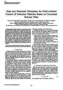
Convergence of θ˜ to zero for various initial conditions.

evolution of error terms x ˜, k˜x , k˜r , θ˜ for the choice of initial conditions given by xm (0) = 20, x(0) = −100, kx (0) = ˆ −200, kr (0) = 200, θ(0) = d−20 20cT . The control parameters in (14) are chosen as k = 10 and α = 0.9. It is evident from the figure that the error terms converge to zero as t → 30 sec.

A. Finite-time online estimation

40

For the parameter estimation scheme presented in Section II, we chose an arbitrary value of θ = −1881 and simulate (9) for various initial conditions for the case when the input u(t) is given as per Figure 1. Figure 2 shows the

20

xm x

x(t)

0

1

5

-20

0

-40

-5

-60 -10

0.8

-80 -100 0

u(t)

0.6

28

28.5

29

29.5

30

Time [sec]

5

10

15

20

25

30

35

40

Time [sec] 0.4

Fig. 3. FTS MRAC: System trajectory x(t) and reference trajectory xm (t). 0.2 300

0 0

1

2

3

4

5

6

7

8

9

10

200

Input signal u(t) for t ∈ [0, 10].

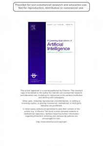
˜ trajectories of θ(t) for various initial conditions θ(0) and for δ = 0.67, ∆ = 1, k1 = k2 = 10, α1 = 0.8, α2 = 1.2. It can be seen that error θ˜ converges to zero within T ≤ 15. B. FTS MRAC We simulate the Case 2, i.e., the system with the disturbance f (x). We choose am = −1, bm = 2, a = 100 and b = 50 so that kx∗ = −2.02 and kr∗ = 0.04. We choose the same reference signal that was used in [16], i.e. r(t) = 5 cos(t) + 10 cos(5t), while the disturbance term is chosen  T as f (x) = θ T ψ, where ψ = x sin(5x) x2 cos(x) and θ = d10 − 10cT . Figure 3 plots the system trajectory x(t) and the reference trajectory xm (t). Figure 4 illustrates the

Error terms

Time [sec] Fig. 1.

x ˜ k˜x k˜r θ˜1 θ˜2

100 0 -100 -200 -300 0

5

10

15

20

25

30

35

40

Time [sec] Fig. 4.

˜x , k ˜r , θ˜ with time t. FTS MRAC: Error terms x ˜, k

C. FTS Adaptive backstepping We simulate the case of n = 2. The reference trajectory is chosen as xr (t) = sin(t) + 0.1t while the unknown parame-

 T ters are chosen as θ = −5 1 and b = 10. The functions  T φi and ψi are chosen as φ1 = x1 sin(x1 ) cos(x1 ) ,  T φ2 = x1 x2 sin(x1 + x2 ) x2 cos(x1 + x2 ) , ψ1 = x1 cos(x1 ) and ψ2 = x2 sin(x1 x2 ). The control gains are fixed as k1 = 10, k2 = 20 while the exponent α is chosen as α = 0.98. The parameter estimation gains are chosen as γp = 10, γθ = 10. Figure 5 shows the system trajectory x(t) and the reference trajectory xr (t) and it can be seen that the closed-loop trajectory tracks the unbounded reference in finite time. Figure 6 shows the error terms e1 , p˜, θ˜1 , θ˜2 starting from initial condition x1 (0) = 10, x2 (0) = 1, pˆ(0) = 1, θˆ1 (0) = 5, θˆ2 (0) = 10. It is evident from the figure that all error terms converge to zero as t → 15. 10 x1 xr

8

x(t)

2 0

x(t)

6 4

-2 5

10

15

Time [sec]

2 0 -2 0

10

20

30

40

50

Time [sec] Fig. 5. FTS Adaptive Backstepping: The state x1 (t) and reference trajectory xr (t) with time t. 15 e1 p˜ θ˜1 θ˜2

Error terms

10 5 0 -5 -10 -15 0

10

20

30

40

50

Time [sec] Fig. 6. FTS Adaptive Backstepping: Error terms e1 , θ˜1 , θ˜2 , p˜ with time t.

VI. C ONCLUSIONS AND F UTURE W ORK In this paper, we presented a novel scheme of online parameter estimation under relaxed persistence of excitation condition with guarantees on convergence of the estimation error in finite time. We designed a novel MRAC with finitetime convergence guarantees for both state- and parametererror in the presence of a class of matched parametric disturbance. We also considered a general class of strict-feedback systems with unknown parameters and designed an adaptive backstepping based finite-time stabilizing control which guarantees both tracking- and parameter-error convergence in

finite time. In future, we would like to investigate methods of finite-time control design for adaptive systems with relaxed or no assumptions on the persistency of excitation. Future work also involves investigating the minimal set of system properties needed to be known in order to be able to design a finite-time stabilizing controller. R EFERENCES [1] P. A. Ioannou and J. Sun, Robust Adaptive Control. Dover Publication, 2012. [2] S. Sastry and M. Bodson, Adaptive Control: Stability, Convergence, and Robustness. Dover Publication, 2011. [3] M. Krsti´c, I. Kanellakopoulos, and P. V. Kokotovi´c, Nonlinear and Adaptive Control Design. John Wiley and Sons., 1995. [4] E. Ryan, “Finite-time stabilization of uncertain nonlinear planar systems,” in Mechanics and control. Springer, 1991, pp. 406–414. [5] S. P. Bhat and D. S. Bernstein, “Finite-time stability of continuous autonomous systems,” SICON, vol. 38, no. 3, pp. 751–766, 2000. [6] ——, “Geometric homogeneity with applications to finite-time stability,” Mathematics of Control, Signals, and Systems (MCSS), vol. 17, no. 2, pp. 101–127, 2005. [7] A. Polyakov, “Nonlinear feedback design for fixed-time stabilization of linear control systems,” IEEE Transactions on Automatic Control, vol. 57, no. 8, p. 2106, 2012. [8] W. S. Black, P. Haghi, and K. B. Ariyur, “Adaptive systems: History, techniques, problems, and perspectives,” Systems, vol. 2, no. 4, pp. 606–660, 2014. [9] E. Cruz-Zavala, E. Nu˜no, and J. A. Moreno, “On the finite-time regulation of euler-lagrange systems without velocity measurements,” IEEE Transactions on Automatic Control, pp. 1–1, 2018. [10] Y. Hong, H. O. Wang, and L. Bushnell, “Adaptive finite-time control of nonlinear systems,” in Proceedings of the 2001 American Control Conference, vol. 6. IEEE, 2001, pp. 4149–4154. [11] Y. Hong, J. Wang, and D. Cheng, “Adaptive finite-time control of nonlinear systems with parametric uncertainty,” IEEE Transactions on Automatic control, vol. 51, no. 5, pp. 858–862, 2006. [12] J. A. Moreno and E. Guzman, “A new recursive finite-time convergent parameter estimation algorithm,” IFAC Proceedings Volumes, vol. 44, no. 1, pp. 3439–3444, 2011. [13] V. Adetola and M. Guay, “Finite-time parameter estimation in adaptive control of nonlinear systems,” IEEE Transactions on Automatic Control, vol. 53, no. 3, pp. 807–811, April 2008. [14] H. Ros, D. Efimov, J. Moreno, and W. Perruquetti, “Finite-time identification algorithm based on time-varying homogeneity and lyapunov approach,” IFAC-PapersOnLine, vol. 49, no. 18, pp. 434–439, 2016. [15] P. Oliva-Fonseca, J. G. Rueda-Escobedo, and J. A. Moreno, “Fixedtime adaptive observer for linear time-invariant systems,” in Decision and Control (CDC), 2016 IEEE 55th Conference on. IEEE, 2016, pp. 1267–1272. [16] E. Guzman and J. A. Moreno, “A new finite-time convergent and robust direct model reference adaptive control for siso linear time invariant systems,” in 2011 50th IEEE Conference on Decision and Control and European Control Conference, Dec 2011, pp. 7027–7032. [17] J. Na, M. N. Mahyuddin, G. Herrmann, X. Ren, and P. Barber, “Robust adaptive finite-time parameter estimation and control for robotic systems,” International Journal of Robust and Nonlinear Control, vol. 25, no. 16, pp. 3045–3071, 2015. [18] Z. Zhu, Y. Xia, and M. Fu, “Attitude stabilization of rigid spacecraft with finite-time convergence,” International Journal of Robust and Nonlinear Control, vol. 21, no. 6, pp. 686–702, 2011. [19] Z. Yu, Y. Yang, S. Li, and J. Sun, “Observer-based adaptive finite-time quantized tracking control of nonstrict-feedback nonlinear systems with asymmetric actuator saturation,” IEEE Transactions on Systems, Man, and Cybernetics: Systems, no. 99, pp. 1–12, 2018. [20] Y. Sun, B. Chen, C. Lin, and H. Wang, “Finite-time adaptive control for a class of nonlinear systems with nonstrict feedback structure,” IEEE Transactions on Cybernetics, vol. 48, no. 10, pp. 2774–2782, Oct 2018. [21] J. Zhou and C. Wen, Adaptive backstepping control of uncertain systems: Nonsmooth nonlinearities, interactions or time-variations. Springer, 2008.