Parameter Estimation of Single and Decentralized Control ... - CiteSeerX

Parameter Estimation of Single and Decentralized Control Systems

Bull. Korean Chem. Soc. 2003, Vol. 24, No. 3

279

Parameter Estimation of Single and Decentralized Control Systems Using Pulse Response Data Eduard Cheres* and Lev Podshivalov Planning Development and Technology Division, The Israel Electric Corp. Ltd., P.O. Box 10, Haifa 31000, Israel Received February 24, 2002 The One Pass Method (OPM) previously presented for the identification of single input single output systems is used to estimate the parameters of a Decentralized Control System (DCS). The OPM is a linear and therefore a simple estimation method. All of the calculations are performed in one pass, and no initial parameter guess, iteration, or powerful search methods are required. These features are of interest especially when the parameters of multi input-output model are estimated. The benefits of the OPM are revealed by comparing its results against those of two recently published methods based on pulse testing. The comparison is performed using two databases from the literature. These databases include single and multi input-output process transfer functions and relevant disturbances. The closed loop responses of these processes are roughly captured by the previous methods, whereas the OPM gives much more accurate results. If the parameters of a DCS are estimated, the OPM yields the same results in multi or single structure implementation. This is a novel feature, which indicates that the OPM is a convenient and practice method for the parameter estimation of multivariable DCSs. Key Words : Parameter estimation, Time delay, Least squares estimation, Linear algorithm, Decentralized control system

Introduction Identification of transfer functions models is required for the tuning and design of controllers. For this purpose, a model of the process is assumed and its parameters are evaluated from a test response data. It has been recognized1 that most process dynamics may in general be simplified by the first order plus dead time (FOPDT) model as: – sh

km e G ( s ) = --------------- ; k m > 0 bs + 1

(1)

or by the second order plus dead time (SOPDT) model as: – sh

km e - ; km > 0 G ( s ) = ----------------------------(2) 2 as + bs + 1 Thus many estimation methods are found in the literature for the parameter estimation (PE) of FOPDT and SOPDT models.2 To enhance the accuracy of the results nonlinear search algorithms are used. But this partially prevents their usage as on-line and on site method. Moreover, it has been recognized that the main problem concerned with the delay estimation with prediction error techniques is due to the multimodal nature of the loss function to be minimized with respect to delay.3 Thus an incorrect guess may results with inadequate estimation. The problem is more complicated if one realized that the estimated delay is not necessarily the true one, i.e. the one measured directly from the pulse response, but rather one of the four parameters which minimize the loss function in question. *

To whom correspondence should be addressed. E-mail: edi@ iec.co.il

Only recently a method which is simple, accurate and free from the above drawbacks was proposed.4 The method is called OPM because the estimation is performed in one pass. The OPM is, to the best of our knowledge, a novel application of linear and non-recursive Least Squared (LS) identification in the frequency domain.5,6 Due to its salient features the results of the OPM were extensively compared4,7,8 with other methods. However all of these comparisons were performed using only step response tests. Hence, It is important and interesting to investigate the OPM results using another popular test signal. A useful and practical test for obtaining experimental dynamic data from many chemical engineering processes is pulse testing. This test signal does not generate an output offset and the test time is relatively short. Due to these features estimation methods using pulse test signal continuously appear in the literature.2,9 Modeling issues associated with multi-input, multi-output (MIMO) systems have long been a significant focus of attention. Even when a proposed MIMO identification is technically sound, ease of use consideration remain a pressing issue to engineering practice.10 The coupling between the system loops degrade the identification results, and as a consequence far fewer investigation were done for MIMO system as compared with single input single output one.9 Therefore, there is great incentive for developing “simple and convenient” ways to accomplish system identification and subsequent control design when the intended application is multivariable control.10 In this content the application of the OPM to MIMO systems with decentralized controllers is investigated. We compare the results of the OPM with those of two state

280

Bull. Korean Chem. Soc. 2003, Vol. 24, No. 3

Eduard Cheres and Lev Podshivalov

of the art methods. These two methods are applied in open and closed loop structures and were especially designed for pulse response data. The bases for the comparison are composed of four single input single output (SISO) dynamics and one MIMO process.2,9 Thus the performances of the OPM with pulse data response and MIMO/SISO structures are thoroughly investigated in this paper. The paper is organized as follows. In the next section the OPM is derived and the state of the art methods based on pulse testing are briefly presented. The comparison between the methods is carried out in open loop and with four representative SISO dynamics. The results of the estimation of the parameters of a MIMO DCS model are presented next, and finally the last section deals with the conclusions.

x ∑ ω f( j ω) + u ∑ ω f( jω) + z ∑ ω f( jω) 8

ω

= ∑ ω f(jω )

kme G ( j ω ) = -------------------------------2 1−a ω + jb ω Thus the LS estimator of the squared amplitude is:

(3)

2

(4)

2

1 2 f ( j ω ) − ------------------------------------------------------2 2 a – 2a- 2 1 ----- ω 4 + b---------------ω + -----2 2 2 km km km

(5)

The following substitution of variables is now in order: 2

b – 2a 1 a - ; z = -----2 x = -----2 ; u = ---------------2 km km km

(6)

Therefore:

ω

1 2 f ( j ω ) − --------------------------------4 2 xω + uω + z

2

(7)

The estimator is nonlinear in the parameters. To make it linear we follow Levy's idea5 and multiply each term in the summation by the denominator of the right hand side term. The original loss function becomes: J L = ∑ [ x ω f ( j ω ) + u ω f ( j ω ) + z f ( j ω ) − 1 ] (8) 4

2

2

2

2

2

ω

The minimum of the loss function is obtained if the following relations hold:

∂ JL ∂J ∂J -------- = 0; -------L- = 0; -------L- = 0 ∂x ∂u ∂z and these result with the equations:

ω

(9a)

x ∑ ω f( j ω) + u ∑ ω f( jω) + z ∑ ω f( jω) 6

4

4

ω

4

2

ω

= ∑ ω f(jω ) 2

(9b)

ω

x ∑ ω f( j ω) + u ∑ ω f( jω) + z ∑ f( j ω ) 4

4

2

ω

4

ω

= ∑ f(j ω )

4

ω

2

4

ω

2

(9c)

ω

km = z

– 0.5

0.5

2

; a = k m x ; b = ( uk m + 2a )

0.5

(10)

A linear LS phase estimator is now defined: ω

where: f( jω) is the frequency response data, which is calculated from the pulse test time response. After some modification one obtains:

JA = ∑

4

2

J P = ∑ [arg f( jω) + hω + arg(1−aω2 + jbω)]2

ω

2

4

ω

–jω h

ω

4

ω

4

We rewrite the SOPDT model in the frequency domain as:

JA = ∑

6

From these linear equations x, u, z are obtained and using Eq. (6) we get:

OPM Parameter Estimation

2 2 JA = ∑ [ f ( j ω ) – G ( j ω ) ]

4

(11)

And this yields the dead time expression:

∑ [ arg f ( j ω ) + arg ( 1 – a ω 2 + jb ω ) ] ω ω

h = − ---------------------------------------------------------------------------------------------∑ ω2

(12)

ω

Remarks: 1. The method6 can be used to generate and calculate the frequency response data. 2. If the identified process is of a higher order the arguments which minimize Eq. (8) do not minimize Eq. (7). In this case the model obtained via the minimization of Eq. (8) is weighted towards the high frequencies.5 Thus we select the critical frequency as the upper limits for the frequency summation in Eq. (9). This forces the model to be skewed towards this critical frequency. A novel features if “identification for control” is sought.10 3. A fairly pedestrian approach is taken to derive the OPM algorithm for a DCS. The extension relay on the linear properties of the method and is explained in details in latter on. If one follows the same lines as for the second order model and use a = 0, the following matrix equation is obtained for the FOPDT parameter estimation: 4 4 2 4 2 2 ∑ ω f ( jω ) ω f ( j ω ) u = ∑ ω f ( j ω )

ω

ω f ( jω ) 2

4

f(jω )

4

z

ω

f (j ω )

(13)

2

km and b are then calculated from Eq. (10). The dead time estimation is also easily obtained as:

∑ [ arg f ( jω ) + arg ( 1 + jb ω ) ] ω ω

h = − -----------------------------------------------------------------------------∑ ω2 ω

(14)

Parameter Estimation of Single and Decentralized Control Systems

Two Comparative Methods Based on Pulse Response Data

(15)

The values of the parameters of the model (see Eq. (2)), which minimize the cost given by Eq. (15), are the estimated ones. The minimization is conducted through the MATLAB11 function “fmins”. Note that the procedure requires initial values of the model parameters, and it is claimed that any reasonable values are good for the initial guess. Parameter Estimation of a DCS in a Closed Loop Configuration (CLC). This method is applicable for multivariable decentralized systems. It is assumed that the DCSs are well defined for the control structure, therefore no “gain directionality” problem12 is associated with these systems. The estimation test is performed with all of the processes in closed loops. A pulse change is sequentially applied to each set-point while the others are kept constant. The following matrix function is then derived: –1 ˆ – 1 –1 Pˆ = [ Rˆ Yˆ − ˆI ] C

(16)

ˆ are respectively: the Laplace transform where: Yˆ , Pˆ , Rˆ , C of the outputs, the process matrix transfer functions, diagonal matrix of the Laplace transform of pulse set point changes, and diagonal matrix of control matrix transfer functions. The Fourier transform of Eq. (16) is the ‘estimation data’. These data is used to estimate a matrix model of FOPTD transfer functions. The estimation loss function is defined for each element (m, n) of the matrix model as follows:

Results of Estimation in Open Loops Four example processes are used for the performance test of the OPM estimation in open loops, and the results are compared against the OLM ones. The transfer functions of the processes are as follow2: –3s

e 1 - ; P 2 ( s ) = ------------------5 ; P 1 ( s ) = -------------------------------------2 ( s + 1 ) ( 2s + 1 ) (s + 1) –s –s e e --------------------------------------------------; ; P P 3 ( s ) = --------------------------------s = ( ) 4 2 2 9s + 2.4s + 1 ( 2s + 2s + 1 ) ( s + 1 ) (18) A common practice is to choose the sampling frequency as 10 to 30 times13 the equivalent time constant inverse. In this example a synthesis of a proportional, integral and derivative (PID) controller is desired. Since a PID controller can achieve a high bandwidth frequency,14 a sampling rate of 6 cycles/min is selected. A square pulse of a height of 1 and a width of 1 [min] is applied2 to all four-example processes. With the OLM one has to select an initial guess for the parameters, and the location of the second data point. We take the second point2 p2 at t = 10 [min], and try two initial guesses for the estimated parameters (marked 1, 2). We select these initial guesses to be symmetric around the previously estimated values.2 Our results are designated as OLMn1 and OLMn2, and are presented in Tables 1-4. The n subscript stands for the level of the noise, which is injected at the process output. For the OPM initial conditions are not required, therefore one subscript (n) is sufficient to designate our results with this method. The estimated models are used in a PID controller synthesis.2 Thus the integral of absolute difference (IAD) between the designed closed loop response and the true one is considered as a relevant quality measure for the quality of the PE. The closed loops responses to a combined disturbance and set point unit steps are simulated, and the IADs are calculated up to 25 [min]. The values of the IADs are presented in Table 3 for the P3(s) process. This process is a true SOPDT process, and a perfect estimation should lead to a zero IAD in the noise free case. However a difference of 116% is found between the IADs of the OLMs with a noise level of zero, and a difference of 114% for the noise level of one. Thus, the OLM results highly depend on the initial guess. With the OPM we first calculate the open loop frequency ratio for the various noise levels. The process frequency response for pulse input is calculated as follows6: ∞

2

ˆ J C ( m,n ) = ∑ Pˆ m, n ( j ωi ) – G m, n ( j ω i )

281

used to find the three model parameters via the JC(m, n) minimization. This is again conducted by the “fmins” function. Again an initial guess of the parameters is required.

In order to investigate the relative advantages of the OPM it is compared with the two state of the art methods. The comparison is carried out by a simulation study over a large number of system dynamics, which were previously selected and used for this purpose. All the relevant aspects of the pulse selection and related noise disturbances are already included in the bases and therefore reflected in the simulation results. Thus a full and a compressive study is performed, eliminating the chance that the results are ‘only a fluke of luck’. In the sequel a brief description of the two state of the art methods is given. For further details the reader is directed to the relevant references.2,9 Open Loop Method (OLM). To apply this method, a square pulse is introduced at the process input and a pulse response is recorded in a relatively short time period. Two points (p1, p2) of the pulse time response are used in the estimation process. p1 is selected as the first peak of the pulse response, whereas p2 is arbitrarily chosen. The estimation loss function is defined as follows: d d J O = p 1 – p 1m + p 2 – p2m + ----- p 2 ( t ) – ----- p 2m ( t ) dt dt

Bull. Korean Chem. Soc. 2003, Vol. 24, No. 3

(17)

i =1

The two frequencies in Eq. (17) are arbitrarily chosen and

j ω ∫ y ( t )e dt 0 f ( j ω ) = --------------------------------------– jω D H(1 – e ) – jω t

(19)

The number of frequency points to be calculated is a

282

Bull. Korean Chem. Soc. 2003, Vol. 24, No. 3

Eduard Cheres and Lev Podshivalov

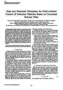
matter of ‘curve fitting’ technique. For a second order system three points of the amplitude frequency graph are required to fix the values of the three parameters (km, a, b). If noise is present two more frequency points are needed to designate the noise parameters. To be on the safe side the points number is doubled. Ten points of frequency are then calculated in the interval (0, Critical frequency]. These points are used in Eqs. (9), (10), (12) to calculate the values of the parameters. As stated the P3(s) process is a SOPDT one, therefore the estimation results can be directly compared against the true ones. The f( jω) points of this process are depicted in Figure 1 against the Bode plot of the model. The match is tight and no difference can be observed between the data points and the relevant Bode points of the OPM0 model. It is obvious from the data in Table 3 that the results of the OPM are the closest to the true ones, and are the less sensitive to the noise. In order to emphasize the relative improvement of the OPM as compared with another method (i), we define the relative improvement of the IAD value as: IAD i – IAD OPM RIADi = ---------------------------------------0 IAD i

(20)

where IAD OPM0 is the closed loop IAD between the response of the OPM model of zero noise and the true one. The RIADs are computed and added to Tables 1, 2 and 4. The RIAD values clearly demonstrate the major improvement obtained with the OPM. This is further demonstrated in Figure 2. where the various P1(s) model responses in the closed loop are depicted against the true one. Obviously the OPM0 response is almost the same as the true one, whereas the OLM ones significantly differ from it. The noise influence can be detected by the RIAD difference between the 0 noise level case and the 1 noise level. From Tables 1, 2 and 4 the additional average for the OPM is 18% as compared to an average of 81% for the OLM. For the true SOPDT process the RIAD resolution is very poor. Therefore

instead of the RIAD the IAD values are presented in Table 3. Again, the OPM-IAD values are much smaller than the OLM ones. Table 1. Estimation results of P 1 ( s ) Method OLM01 OLM02 OPM0 OLM11 OLM12 OPM1

Noise STD Level 0

0

1

0.01

km

a

b

h

RIAD

0.989 1.283 1.000 1.035 0.955 0.982

1.374 4.545 3.181 2.573 2.804 3.549

2.344 4.264 3.505 3.208 3.349 3.648

2.867 2.312 3.503 1.047 4.151 3.378

97.9 96.6 00.0 98.0 95.8 23.0

Notes: A. Initial conditions for OLMn1 are - km = 0.5 a = 2 h = 2. B. Initial conditions for OLMn2 are - km = 1.5 a = 5 b = 4.5 h = 4. C. STD-standard deviation of a Gaussian noise with zero mean. D. RIAD\PID settings (KC = 0.931, JI = 4.34 JD = 1.54)

Table 2. Estimation results of P 2 ( s ) Method OLM01 OLM02 OPM0 OLM11 OLM12 OPM1

Noise STD Level 0

0

1

0.01

km

a

b

h

RIAD

0.524 0.824 0.998 0.524 0.927 1.010

1.729 2.012 3.753 1.729 2.340 3.785

2.630 3.155 3.469 2.630 3.438 3.566

0.861 2.568 1.551 0.861 2.470 1.506

81.1 70.9 0.0 81.0 71.3 6.3

Notes: A. Initial conditions for OLMn1 are - km = 0.5 a = 1.5 b = 2 h = 1. B. Initial conditions for OLMn2 are - km = 1.5 a = 4.5 b = 4.5 h = 2. C. RIAD\PID settings (KC = 1.41, JI = 3.50 JD = 1.50).

Table 3. Estimation results of P 3 ( s ) Method OLM01 OLM02 OPM0 OLM11 OLM12 OPM1 True values

Noise Level

STD

0

0

1

0.01

km

a

b

0.961 11.111 1.711 1.097 7.671 3.209 0.996 9.019 2.387 0.753 7.152 1.080 1.252 7.644 3.721 0.992 9.190 2.387 1.000 9.000 2.400

h

IAD

0.305 1.578 1.002 0.927 1.535 0.957 1.000

1.193 2.588 0.022 1.354 2.903 0.073 0.00

Notes: A. Initial conditions for OLMn1 are - km = 0.5 a = 6 b = 2 h = 0.8. B. Initial conditions for OLMn2 are - km = 1.5 a = 12 b = 4 h = 1.5. C. IAD\PID settings (KC = 1.95, JI = 3.33 JD = 3.02).

Table 4. Estimation results of P 4 ( s ) Identification Noise STD Method Level OLM01 OLM02 OPM0 OLM11 OLM12 OPM1

Figure 1. Frequency response data points of P3(s) against the Bode plot of its OPM0 model.

0

0

1

0.01

km

a

b

h

RIAD

0.578 0.437 0.999 1.119 0.690 1.010

0.818 0.251 2.388 6.712 0.827 2.177

1.425 1.097 2.367 2.363 1.818 2.381

2.620 3.014 1.649 0.458 2.587 1.689

74.6 80.2 00.0 72.0 67.1 23.7

Notes: A. Initial conditions for OLMn1 are - km = 0.5 a = 2 b = 1 h = 1. B. Initial conditions for OLMn2 are - km = 1.5 a = 6 b = 4 h = 2. C. RIAD\PID settings (KC = 1.15, JI = 2.01 JD = 1.69).

Parameter Estimation of Single and Decentralized Control Systems

Figure 2. True and estimated closed loop responses of P1(s) with a series PID controller (kc = 0.931, τI = 4.34, τD = 1.54).

Bull. Korean Chem. Soc. 2003, Vol. 24, No. 3

If the “fmins” routine is used to minimize this cost function, it results with negative delays and negative time constants. Therefore an optimization with zero lower bound on the delays and time constants is applied, and is carried out via the MATLAB “constr” function. Two sets of initial conditions are used, and the results are designated CLC1 and CLC2. These results are depicted in Table 5 and the associated initial conditions are presented in Table 6. It can be observed that the CLC1 values for Pˆ 1,3 and Pˆ are 2,3 approximately half of those obtained with the CLC2. Moreover, using the single estimator of Eq. (17) another values were obtained9 for the parameters of the distillation model. Returning to the OPM, a global amplitude loss function is introduced as follows: J A = ∑ J A ( m,n )

Results of Estimation in Closed Loops

J C = ∑ J C ( m,n ) m, n

(22a)

m, n

The example system is a 3 × 3-distillation dynamics, and the process transfer functions are listed in Table 5. The following test procedure is followed.9 Firstly, decentralized proportional controllers are applied to the dynamics in closed loops. The proportional gains are 1, -0.1 and 1 for loops 1, 2 and 3, respectively. Then, a rectangular pulse having height of one and width of one [min] is applied to the set point of each control loops one at a time and a sampling rate of 0.1 [min] is used. The CLC procedure is now used to obtain the estimation data at the two frequency points9: 0.01 and 0.05 [rad/min]. Instead of minimizing the loss function of Eq. (17) for each system component, we minimize the following global loss function: (21)

where: 2 2 J A ( m,n ) = ∑ [ f m, n ( j ωi ) – G m, n ( j ωi ) ]

2

Actual

Using the same reasoning a global phase estimator is also easily derived. Since any system component (m, n) is independent, the linear LS solution of the global estimator of Eq. (22) is exactly the same as the one for the single estimator, i.e the solution of Eqs. (9)-(10) is repeated for every (m, n) component. The same reasoning is also true for the solution of the global phase estimator. The ‘estimation data’ used with the CLC method is also used with the global OPM estimator, and the estimated parameters are presented in Table 5. Again the OPM results are very close to the true ones (see Table 5 for details). In contrast to the previous results no ambiguousness exists

Estimated CLC1

Pˆ 1,1

0.66e ---------------------6.7s + 1

Pˆ 1,2

0.66 e –------------------------8.64s + 1

Pˆ 1,3

– 0.0049 e ------------------------9.06s + 1

–2.6s

– 3.5s

–s

Pˆ 2, 1

– 1.11e ---------------------3.25s + 1

Pˆ 2, 2

– –2.3 e ------------------5s + 1 1.2s 0.01 e– –------------------------7.09s + 1 9.2s 34.68 e – – ---------------------------8.15s + 1

Pˆ 2, 3 Pˆ 3, 1

6.5s

3s

Pˆ 3, 2

46.2e ---------------------10.9s + 1

Pˆ 3, 3

0.89 ( 11.61s + 1 )e -----------------------------------------------------( 3.89s + 1 ) ( 18.8s + 1 )

–9.4s

–s

CLC2

–2.60 s

0.66e -----------------------6.7s + 1 –3.51s –0.61 e -------------------------8.63s + 1 –1.46 s 0.005 e –----------------------------15.18s + 1 6.50 s 1.11e – ----------------------3.25s + 1 –3.00s –2.30 e -------------------------5.00s + 1 –1.33s –0.01 e -------------------------10.06s + 1 – 9.2s – 34.7 e ------------------------8.2s + 1

–9.3s

46.2e --------------------10.9s + 1 –0.62 s 0.86e -----------------------6.82s + 1

0.66e -----------------------6.7s + 1 –3.51s –0.61 e -------------------------8.63s + 1 –0.70 s – 0.0048 e -------------------------------6.49s + 1 –6.50 s 1.11e -----------------------3.25s + 1 3.00s 2.30 e – –-------------------------5.00s + 1 1.04s 0.01 e – – --------------------------4.66s + 1 9.2s 34.7 e– –------------------------8.2s + 1 46.2e ---------------------10.9s + 1 –0.62 s 0.86e -----------------------6.83s + 1

(22b)

i=1,2

Table 5. Processes and estimated models of a 3 × 3 distillation system Process

283

OPM

–2.60 s

0.66e – -----------------------6.7s + 1 – 3.5s – 0.61 e ------------------------8.63s + 1 – 0.99s 0.0049 e –-------------------------------9.06s + 1 6.49 s 1.11e – ----------------------3.25s + 1 –3.00s –2.29 e -------------------------4.99s + 1 1.19s 0.01 e– –-------------------------7.09s + 1 –9.18 s – 34.68 e ----------------------------8.16s + 1

2.59 s

–9.3s

46.24e --------------------------10.93s + 1 –0.62 s 0.86e -----------------------6.59s + 1

– 9.35s

284

Bull. Korean Chem. Soc. 2003, Vol. 24, No. 3

Eduard Cheres and Lev Podshivalov

Table 6. Initial conditions for the estimation of the distillation system Process

Initial Conditions CLC1

Pˆ 1,1

0.3e– --------------3s + 1

Pˆ 1,2

– –0.3 e ------------------4s + 1

Pˆ 1,3

1s

2s

–0.5s

– 0.002 e ---------------------------6s + 1

CLC 2 4s

1e – -----------------10s + 1 5s

– –1 e ----------------12s + 1 – 1.5 s

–0.007 e ---------------------------15s + 1

Pˆ 2, 1

0.5e– --------------1s + 1

3s

1.5e – -----------------5s + 1

Pˆ 2, 2

– –1 e -----------------2.5s + 1

1.5 s

– –4e -----------------7.5s + 1

Pˆ 2, 3

–0.6s

– 0.005 e ---------------------------4s + 1

Pˆ 3, 1

– – 17 e ----------------4s + 1

Pˆ 3, 2

– 25e --------------5s + 1

Pˆ 3, 3

These highly facilitated the application of the OPM at the plant floor especially with MIMO systems.

5s

10s

4.5s

–1.5s

– 0.02 e ------------------------10s + 1 – 15s

50 e –------------------12s + 1

5s

60e– ----------------15s + 1

– 0.5s

1.5e -----------------10s + 1

0.5e ------------------3s + 1

15s

–1.5s

between the OPM results which are obtained with the single and global estimators. Conclusions The OPM is extended to the MIMO case and it’s results are investigated and compared against two state of the art methods based on pulse testing. The comparison is performed by a simulation study. To remove the chance that the study results are just ‘a fluke of luck’ two comparative test bases from the literature are used. One basis includes four high order SISO dynamics and the second includes a 3 × 3 MIMO process with decentralized controllers in closed loops. In all the cases the OPM results are better than those obtained with the previous methods. The OPM results are also found to be more robust to the measurement noise. As differ from the previous methods, the OPM is linear and it’s results do not depend on an ‘initial guess’ of the parameters. Moreover, the drawback of multiple solutions of the previous methods is removed. It is also shown that the OPM results for a global MIMO estimator are identical to those of several SISO estimators. This outcome is unique to the OPM and is not achieved by any of the previous methods. In other words, a linear algorithm for the explicit solution of the MIMO global estimator is obtained whose calculation burden is equivalent to the one of an SISO estimator.

Nomenclature a : denominator coefficient in eq. 3 b : denominator coefficients in eq. 3 ˆ : diagonal matrix of control transfer functions C D : width of pulse [min] f, fm,n : frequency response data [rad/min] G : transfer function of a process model H : height of pulse h : dead time [min] Iˆ : identity matrix j : fundamental imaginary number JA, JA(m,n) : LS estimators of the squared amplitude JL : Levy estimator JO : OLM estimator JP, JP(m,n) : Phase estimators kc : controller proportional gain km : model gain P : transfer function of a process Pˆ : multivariable process matrix function Pˆ m, n : component of Pˆ p1, p2 : data points from the pulse response curve p1m, p2m : points from the model pulse response curve Rˆ : diagonal matrix of pulse set point changes s : Laplace variable t : time [min] u : assigned variable x : assigned variable y(t) : process output Yˆ : matrix of multivariable outputs z : assigned variable Greek Letters ω : vector of frequency points [ rad/min] τD : controller derivative time [min] τI : controller integral time [min]

References 1. Huang, C.-T.; Chau, C.-J.; Wang, J.-L. J. Chinese Inst. Chem. 1996, 27, 107. 2. Ham, T. W.; Kim, Y. H. Ind. Eng. Chem. Res. 1998, 37, 482. 3. Ferretti, G.; Maffezzoni, C.; Scattolini, R. Automatica 1996, 449. 4. Cheres, E.; Eydelzon, A. Proc. of the Eight. IASTED Int. Conf. Modelling Ident. and Contr.; ACTA Press: Calgary, Canada, 1999; p 483. 5. Schoukens, J.; Pintelon, R. Identification of Linear Systems; Pergamon: Oxford, 1991; p 55. 6. Luyben, W. L. Process Modeling Simulation, and Control for Chemical Engineers; McGraw-Hill: New York, 1990; p 505. 7. Cheres, E.; Eydelzon, A. Process Contr. and Quality 1999, 11, 301. 8. Cheres, E.; Eydelzon, A. Process Contr. and Quality 1999, 11, 307. 9. Ham, T. W.; Kim, Y. H. J. Chem. Eng. of Japan 1998, 31, 941. 10. Rivera, D. E.; Jun, K. S. IEEE Control Systems Magazine 2000, 20, 25. 11. Grace, A. Optimization Toolbox for Use with MATLAB; The MathWorks Inc.: Natick, U.S.A, 1994; pp 3-16. 12. Li, W.; Lee, J. H. AIChE J. 1996, 42, 2813. 13. Lauzi, M. Proc. of the IEMDC ’99 1999, 460. 14. Astrom, K. J. Int. J. of Adaptive Contr. and Signal Processing 1991, 5, 3.