Simultaneous active parameter estimation and control using sampling

Simultaneous active parameter estimation and control using sampling-based Bayesian reinforcement learning

arXiv:1707.09055v1 [cs.SY] 27 Jul 2017

Patrick Slade1 , Preston Culbertson1 , Zachary Sunberg2 , and Mykel Kochenderfer2 Abstract— Robots performing manipulation tasks must operate under uncertainty about both their pose and the dynamics of the system. In order to remain robust to modeling error and shifts in payload dynamics, agents must simultaneously perform estimation and control tasks. However, the optimal estimation actions are often not the optimal actions for accomplishing the control tasks, and thus agents trade between exploration and exploitation. This work frames the problem as a Bayesadaptive Markov decision process and solves it online using Monte Carlo tree search and an extended Kalman filter to handle Gaussian process noise and parameter uncertainty in a continuous space. MCTS selects control actions to reduce model uncertainty and reach the goal state nearly optimally. Certainty equivalent model predictive control is used as a benchmark to compare performance in simulations with varying process noise and parameter uncertainty.

I. INTRODUCTION A. Motivation Flexibility and robustness in real-world robotic systems is essential to making them human-friendly and safe. Planning for important tasks in robotics, such as localization and manipulation, requires an accurate model of the dynamics [1]–[3]. However, the dynamics are often only partially known. For example, order-fulfillment robots move containers with varying loads in warehouses [4], autonomous vehicles traverse variable terrain and interact with human drivers [5]–[7], and nursing robotic systems use tools and interact with people [8]. Payload shifts, environment conditions, and human decisions can dramatically alter the system dynamics. Even for motion determined by physical laws, there are often unknown parameters like friction and inertial properties. In these cases, the robot must estimate the system dynamics to achieve its goals. Unfortunately, this estimation task often conflicts with the original goal task. The robot must balance exploration to gain knowledge of the dynamics and exploitation of its current knowledge to obtain rewards. B. Related Work Often this is solved with certainty equivalent control where a robot plans assuming an exact dynamics model [9]. This is This work is supported by the National Science Foundation Graduate Research Fellowship Program Grant DGE-1656518 and the Stanford Graduate Fellowship. Toyota Research Institute (”TRI”) provided funds to assist the authors with their research but this article solely reflects the opinions and conclusions of its authors and not TRI or any other Toyota entity. 1 P. Slade and P. Culbertson are with the Department of Mechanical Engineering, Stanford University, Stanford, CA 94305 USA (e-mail: {patslade, pculbertson}@stanford.edu). 2 Z. Sunberg and M. Kochenderfer are with the Department of Aeronautics and Astronautics, Stanford University (e-mail: {zsunberg, mykel}@stanford.edu).

usually the most likely or mean dynamics model. Typically, this dynamics model will update every time it receives an observation and make a new plan up to a fixed horizon that is optimal for the updated dynamics model. This approach is known as model predictive control (MPC) [9], [10]. In some cases, performance can improve if a range of dynamic models are considered. This approach is known as robust MPC [11]–[13]. These approaches work well in many cases, however they do not encourage exploration, and are thus suboptimal for some problems [14]. There have been a variety of principled approaches to handle the exploration-exploitation trade-off. One body of research has referred to this challenge as the “dual control” problem [15]. It was shown that an optimal solution could be found using dynamic programming (DP). However, since the state, action, and belief spaces are continuous, the exact solution is generally intractable. Approximate solutions include a variety of methods such as adaptive control, sliding mode control, and stochastic optimal control [16]. Adaptive controllers typically first perform an estimation task to reveal unknown parameters and then perform the control task. This is suboptimal, the agent could potentially use the estimation actions to also begin performing the control task. Another popular approach is reinforcement learning (RL) [17]. In RL, the underlying planning problem is a discrete or continuous Markov decision process (MDP) with unknown transition probability distributions. RL agents interact with the environment to accrue rewards and may learn the transition probabilities along the way if it helps in this task. If the prior distribution of these transition probabilities is known, the policy that will collect the most reward in expectation, optimally balancing exploration and exploitation, may be calculated by solving a Bayes-adaptive Markov decision process (BAMDP) [18]. Unfortunately BAMDPs are, in general, computationally intractable, so approximate methods are used [19]. Since any BAMDP can be recast as a partially observable Markov decision process (POMDP), similar approximate solution methods are used. Both offline [20] and online [19] POMDP methods have been used for RL in discrete state spaces, and others [21] are easily adapted. There has been limited work on continuous spaces. Value iteration has been used for problems with Gaussian uncertainty [22]. Controls are locally optimized along a precomputed trajectory as an extended Kalman filter (EKF) updates the belief over the model parameters. Exploration is encouraged by heuristically penalizing model uncertainty in the reward function. The control designer chooses how much to explore rather than the algorithm optimally calculating it.

C. Contribution This research applies Monte Carlo tree search (MCTS) to solve a close approximation to the BAMDP for a problem with continuous state, action, and observation spaces, an arbitrary reward function, Gaussian process noise, and Gaussian uncertainty in the model parameters. An EKF updates the belief of the unknown parameters and double progressive widening (DPW) [23] guides the expansion of the tree in continuous spaces. Section II gives an introduction to the problems and methods considered, Sections III and IV give detailed descriptions of the problem and approach, and Section V shows simulations comparing MCTS with a certainty-equivalent MPC benchmark for two problems. II. BACKGROUND This section reviews techniques underlying our work: sequential decision making models, MCTS, and EKFs. A. MDPs, POMDPs, BAMDPs A Markov decision process is a mathematical framework for a sequential decision process in which an agent will move, typically stochastically, between states over time, accruing various rewards for entering certain states, but may affect their trajectory and rewards by taking actions at each time step. A MDP is defined by the tuple (S, A, T, R, γ), where: • • • • •

S is the set of states the system may reach, A is the set of actions the agent may take, T (s0 | s, a) is the probability of transitioning to state s0 by taking action a at state s, R(s, a) is the reward (or cost) of taking action a at state s, and γ ∈ [0, 1] is the discount factor for future rewards.

Solving an MDP develops a policy, π(s) : S → A, which maps each state to an optimal action that will accrue the most rewards in expectation over some planning horizon. For infinite-horizon, discounted MDPs, the optimal policy has been shown to satisfy the Bellman equation [9]. For small, discrete state and action spaces, the Bellman equation may be solved explicitly with DP. However, for problems with large or continuous state and action spaces approximate solutions use approximate DP (ADP) [24]. Next, we discuss MCTS, the online ADP algorithm applied in this work. A partially observable MDP (POMDP) is an extension of an MDP, where the agent cannot directly observe its true state, only receiving observations which are stochastically dependent on this state. A POMDP thus contains a model of the probability of seeing a certain observation at a specific state. The agent forms a belief state, b which encodes the probability of being in each state s. The agent updates its belief at each step, depending on its previous action, the reward received, and the observation it took. Since the agent may hold any combination of beliefs about its location in the state space, the belief space B is continuous, making POMDPs computationally intensive to solve.

A Bayes-adaptive MDP (BAMDP) has transition probabilities that are only partially known. That is, the decisionmaking agent initially only knows a prior distribution of the transition probabilities. As the agent interacts with the environment, it extracts information of the transition probabilities from the history of states and actions that it has visited. A BAMDP becomes a POMDP by augmenting the state with the unknown parameters defining the transition probabilities. A POMDP is actually an MDP where the state space is the belief space of the original POMDP [14], sometimes called a belief MDP. The transition dynamics of the belief MDP are defined by a Bayesian update of the belief when an action is taken and an observation received. Not all belief MDPs are POMDPs; in a POMDP, the reward function is specified only in terms of the POMDP state and action and is not a general function of the belief, so penalties cannot be explicitly assigned to uncertainty in the belief. When the belief update is computationally tractable, ADP techniques designed for MDPs may be applied to POMDPs by applying them to the corresponding belief MDP. B. Monte Carlo Tree Search MCTS is a sampling-based online approach for approximately solving MDPs. MCTS uses a generative model G to get a random state and reward (s0 , r) ∼ G(s, a). It performs a forward search through the state space, using G to draw prospective trajectories and rewards. In MCTS, a tree is created with alternating states and actions, with a roll-out performed to select a policy [25]. In general, MCTS involves stages: selection, expansion, rollout, and propagation [26]. C. Extended Kalman Filter In problems with linear Gaussian dynamics and observation functions, it has been shown that the optimal observer is a Kalman filter. A Kalman filter is an iterative algorithm that can exactly update Gaussian beliefs over the state, given the action taken, the observation received, and the transition and observation models [3]. For systems with nonlinear dynamics, an EKF may be used to approximately update the beliefs with each step [3]. Let xk , ak , and ok be the state, action, and observation at time t = k. For a system with nonlinear-Gaussian dynamics, the transition and observation models can be expressed as xk+1 = f (xk , ak ) + vk

(1)

ok = h(xk , ak ) + wk ,

(2)

where f , h are nonlinear functions and v, w are normally distributed. The Gaussian belief has mean x ˆ and covariance Σ. The EKF updates the belief at each timestep by predicting a new state and covariance based on the action taken, i.e. x ˆk|k−1 = f (ˆ xk−1|k−1 , ak−1 )

(3)

T Σk|k−1 = Fk−1 Σk−1|k−1 Fk−1 + Qk−1 ,

(4)

where F is the linearized dynamics about the current belief. ∂f (5) Fk−1 = ∂x xˆk−1|k−1 ,uk−1

where v˜ ∼ N (0, diag(Q, P )) and P is a parameter drift matrix. The observation model is described by   ok = C(p) 0 sk + D(p)uk + wk . (18)

A residual between the observation and predicted state is:

If we use an EKF to describe the belief about the current state in the state-parameter space, we form a belief MDP over all possible EKF states. This belief MDP is described by the tuple (S, A, T, R), where: • S is the space of all possible beliefs. Since the belief maintained by the EKF is Gaussian, it can be described by the mean and covariance, bk = (ˆ sk , Σk ). • A is all possible actions that the agent may take. 0 • T (b | b, a) is a distribution over possible EKF states after a belief update. This distribution depends on the observation model. It is difficult to represent explicitly, so it is implicitly defined by the generative model, G. • R(b, a) is a reward function for a given belief and action. It is constructed as desired for a given control task. In our work, we approximate R(b, a) = R(ˆ sk , a), a linear reward for the estimated mean state and action. The generative model for the belief MDP is

rk = ok − h(ˆ xk|k−1 , ak−1 ).

(6)

The residual covariance, Sk and Kalman gain, Kk are Sk = Hk Σk|k−1 HkT + Rk

(7)

Kk = Σk|k−1 HkT Sk−1

(8)

where Hk is the linearized observation function. ∂h Hk = ∂x

(9)

x ˆk|k−1 ,uk−1

Finally, the belief update is completed according to x ˆk|k = x ˆk|k−1 + Kk rk

(10)

Σk|k = (I − Kk Hk )Pk|k−1 .

(11)

Due to the linearization of the dynamics and observation models, EKFs will not always converge and are generally not optimal observers. However, in practice they perform well for most systems where the true belief is unimodal. III. P ROBLEM F ORMULATION Let us consider a robot trying to control a system with linear-Gaussian dynamics. The system is described by xk+1 = f (xk , uk ; p) + vk ,

(12)

where xk , uk are the state and control action at time t = k, p is a set of parameters that the system dynamics depend on, the process noise vk ∼ N (0, Q), and f is a time-invariant function that is linear with respect to xk and uk , f (xk , uk ; p) = A(p)xk + B(p)uk .

(13)

The observation model is described by the linear equation ok = h(xk , uk ; p) + wk ,

(14)

with observation, ok taken at time t = k, the measurement noise wk ∼ N (0, R), and h is a time-invariant linear function h(xk , uk ; p) = C(p)xk + D(p)uk .

(15)

While f and h are physical equations known a priori, the parameters p are not known beforehand. They can be appended to the state vector to form a state-parameter vector,   xk sk = . (16) p Thus, the system dynamics for sk may be described by     A(p) 0 B(p) sk+1 = sk + uk + v˜k , (17) 0 I 0

bk+1 = G(bk , ak )

(19)

with G defined by equations (3), (4), (6), (10), and (11). The observation, ok , used in (6) is a random variable determined by (1) and (2); it is not the most likely observation. Solving this belief MDP gives a policy that optimally maximizes the sum of expected rewards over some planning horizon. IV. A PPROACH This section discusses the use of MCTS and MPC with an EKF to control a system with unknown parameters. A. MCTS Our approach uses the upper confidence tree (UCT) [25] and DPW [23] extensions of MCTS. The tree is built as UCT expands action nodes maximizing an upper confidence estimate s ˜ u) + c log N (s) , (20) U CB(s, u) = Q(s, N (s, u) ˜ u) estimates the state-action value function from where Q(s, rollout simulations and tree search, N (s, u) counts the times action u is taken from state s, with exploration constant, c. This balances exploration-exploitation as the tree expands. DPW defines tree growth for large or continuous state and action spaces. To avoid a shallow search, the number of children of each state-action node (s, u) is limited to kN (s, u)α ,

(21)

where k and α are parameter constants tuned to control the widening of the tree. With an increase in N (s, u) the number of children also grows, widening the tree. The number of actions explored at each state is limited similarly.

A large number of nonlinear stochastic systems can be near-optimally controlled with an EKF and MCTS or MPC. The purpose of this method is to produce and execute a control policy. Any system described by a model in the form of (12) with an approximately Gaussian initial belief state can use MCTS or MPC to find a suitable control action. Taking this action propagates the true state, s, which will be partially observed. This observation and action will update the belief state with the EKF, improving our estimates about the parameters. This process is shown in Algorithm 1. Algorithm 1 Simultaneous estimation and control Require: b0 (s), s0 for t ∈ [0, T ) do ut ← P OLICY(bt ) ot ← R ECEIVE M EASUREMENTS(st ) bt+1 ← EKF(bt , ut , ot ) st+1 ← P ROPOGATE DYNAMICS(st , ut ) return ui |Ti=0 D. Implementation Details Measurement noise was removed from the tests so the effects of process noise and estimated parameter uncertainty were isolated. The magnitude of control inputs was limited to umax (see Table I). Filtering the control signal is recommended for experimental validation to not damage actuators. A linear reward function was implemented with a weighted L1 norm penalty for the position, speed, and control effort   Rpos 0 RL1 (xk , uk ) = xk + Ru uk . (22) 0 Rvel The values for Rpos , Rvel , and Ru are given in Table I. For performance comparison purposes a quadratic reward function is used with a L2 norm penalty for the same terms RL2 (xk , uk ) = xTk



Rpos 0

0 Rvel



xk + uTk Ru uk . (23)

Real-world constraints were included as a minimum threshold for physical values such as mass, friction, and inertia so the dynamic models held. The MCTS rollout used a position controller to select a force proportional to the distance from the goal state. The MCTS with DPW implementation is from the POMDPs.jl package [27]. The optimization in the MPC controller was solved with the Convex.jl package [28].

10

0

20

40

60

80

100

0

20

40

60

80

100

0

20

40

60

80

100

20 Velocity (m/s)

C. Basic Approach

MPC MCTS

20

0

Force (N)

MPC is a technique for online calculation of a policy [10]. Its extensive use in control system design is due to its ability to explicitly meet state and control constraints. For our implementation of MPC, the optimization problem is constrained by the dynamics, f (xk , uk , p), and the maximum control effort, umax . At each step a series of control actions to maximize a reward function are found for a fixed horizon from the current state and the first action is taken [9].

Position (m)

B. Model Predictive Control

10 0 −10

200 0 −200

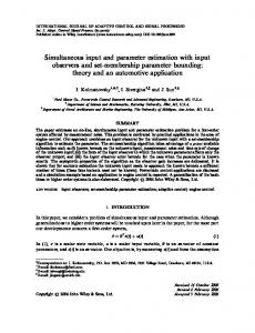
Steps (0.1 seconds) Fig. 1. Position, velocity, and force profiles of the controllers for the 1D double integrator model

V. S IMULATION AND R ESULTS Models of a 1D double integrator and robot performing planar manipulation tested our MCTS approach against MPC, a certainty equivalent optimal control benchmark. A. 1D Double Integrator Model We first considered the control problem where an agent applies force to a point mass in one dimension with dynamics " #   ∆t 1 0 m
xk+1 = xk + f k + vk (24) ∆t 2 ∆t 1 m  ok =

1 0

0 1

 xk + w k .

(25)

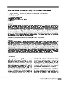
Measurement noise is 0 to reduce the number of parameters. Fig. 1 gives physical intuition to the 1D double integrator model. The point mass starts at a given position and velocity with a goal state at the origin. The state profiles for MCTS appear smoother than MPC. This is due to MPC applying large forces for short duration caused by the large penalty an L1 reward function gives small errors. B. Planar Manipulation (PM) Model We then consider a robot R pushing a box B in the plane, where the agent may apply an arbitrary force in the x- and y-directions, in addition to a torque. This problem, with its related quantities, is illustrated in Figure 2. We can describe the dynamics of the system about its center of mass, Bcm . These are given by X F~B = F~ − µv ~v = m~a (26)

This model uses the same stationary goal at the origin with an orientation of 0 degrees. It is given an initial position and orientation with Cartesian and angular velocities. C. Results

Fig. 2.

Schematic of planar manipulation (PM) task

X

T~B = T~ + ~r × F~ = J α ~,

(27)

where µv is linear friction. The system in discrete-time is vk+1 = ak ∆t + vk

(28)

pk+1 = vk ∆t + pk ,

(29)

where ∆t is the discretization step. The system can be put  in state-space form with the state T vector px,k , py,k , θk , vx,k , vy,k , ωk xk = , corresponding to the linear and angular positions and velocities of B in the global frame N . Using (26) and (27) and an explicit-time integration xk+1 = f (xk , uk ) = Axk + B(θ)uk + vk , where

" A=

I3x3

I3x3 ∆t

03x3

I3x3

   B= 

#

0 B 3,1

0 ∆t m 3,2

B

, 

03x3 ∆t m

(30)

 0  , 0 

∆t J

∆t (cos(θ)ry + sin(θ)rx ), J ∆t = (cos(θ)rx − sin(θ)ry ), J   Fx,k uk =  Fy,k  , Tk

B 3,1 = B 3,2

where m is the mass of B and J is B’s moment of inertia. For a robot with noisy sensors which measure its position, velocity, and acceleration in N , the observation model is yk = h(xk , uk ) + wk ,

(31) T

where yk = [px,k , py,k , θk , vx,k , vy,k , ωk , ax,k , ay,k , αk ] . The measurement functions are given by p~ = ~rcm + ~rb

(32)

~v = ~vcm + ω ~ × ~rb P~ TB α ~= J P ~ FB ~a = +α ~ × ~rb + ω ~ × (~ ω × ~rb ). m

(33) (34) (35)

The simulations performed on both models compare the rewards for MCTS and MPC for two varied parameters: process noise and initial parameter uncertainty. Fig. 3 compares rewards of MCTS and MPC for the 1D double integrator model while varying process noise. The simulation parameters are detailed in Table I. While MPC and MCTS perform similarly for small process noise, the reward accrued by MPC decreases significantly faster as process noise increases. Process noise greater than 1.0 has little impact on the reward, indicating saturation when the process noise is so large the policy cannot reach the goal region. 30 trials were run for each case with standard error of the mean indicated by the error bars. The standard deviation of the initial parameter estimate was then varied for a constant process noise with variance 3.0. This process noise level was chosen because it highlights the rapid change in reward caused by a poorer initial mass estimate. Fig. 4 shows the MCTS reward mostly unaffected by this uncertainty, while the MPC reward decreases rapidly. This highlights the advantage of exploration-exploitation from MCTS. Searching for actions using multiple estimates of the mass and moving towards the goal allows it to get better knowledge of the system and increase reward. MPC takes the first action of an open-loop certainty-equivalent plan recalculated every step. Another interesting topic to consider is the performance of MCTS and MPC considering parameter uncertainty with different reward functions. The relative rewards of MCTS and MPC with linear (L1) and quadratic (L2) reward functions are shown in Fig. 5. In both cases the process noise had variance 1.0 and the initial mass estimate had variance 10.0. While MCTS performs significantly better with an L1 reward, it performs slightly worse with an L2 reward. These results indicate that, with an L2 reward in these domains, taking uncertainty into account with MCTS is not beneficial. This is due to the L2 reward function placing a small penalty on small errors, allowing MPC to perform well without considering parameter uncertainty. In another study with a quadratic state reward [22], the reward function is augmented with a term penalizing parameter uncertainty. We suspect that, without this explicit stimulus to explore rather than simply exploit, planning algorithms would not need to actively gather information about the parameters to perform well in domains with quadratic reward. A chief advantage of the POMDP approach is that the solver automatically gathers information necessary to maximize the reward. Explicit penalization of uncertainty should not be necessary if the state reward function is chosen to accurately reflect the performance requirements. It should be noted that convex reward functions were used to allow easy comparison with MPC, but there is no need for the reward function used by

·105

·105 0

0 −0.2

−1 Total Reward

Total Reward

−0.4 −0.6 −0.8

−2

−1 −1.2

MPC MCTS

MPC MCTS

−3 10−1

100

100

Process Noise (σ)

Fig. 4. Effects of different initial mass estimate standard deviations on reward for the 1D double integrator model

TABLE I S IMULATION PARAMETERS Symbol

Value 1D

Value PM

∆t c k α wk Ru Rpos Rvel

0.1 s 300 8.0 0.2 0.0 −1.0 −10.0 −3.0 20 4.0 2000 20 300.0 100 30 10.0 1.0

0.1 s 100 8.0 0.2 0.0 −0.1 −1.0 −1.0 20 8.0 10, 100 20 100.0 100 30 10.0 1.0

n umax

·105

·105

Total Reward

Time step UCT exploration parameter DPW linear parameter DPW exponent parameter Measurement noise Reward scaler for force Reward scaler for position Reward scaler for velocity MCTS search depth Position roll-out gain MCTS-DPW iterations per step MPC horizon Magnitude of force range Steps per trial Trials per test case Initial parameter estimate variance Parameter and estimate lower bound

102

Initial Mass Estimate (σ)

Fig. 3. Effects of different levels of process noise on reward for the 1D double integrator model

Parameter

101

0

0

−0.2

−0.2

−0.4

−0.4

−0.6

−0.6

−0.8

−0.8

−1

−1

−1.2

−1.2

0.5

MCTS to be convex. Designers can use reward functions that precisely prescribe the desired behavior. The simulation for varying process noise in the PM model is displayed in Fig. 6. It behaves like the 1D model; MCTS has higher reward for all noise levels. As iterations per step decreases, MCTS tracks closer to MPC. This smaller reward difference than in the 1D case indicates the EKF has trouble reducing uncertainty for five estimated parameters in a nonlinear and time-varying system. Thus, rewards decrease with increasing process noise for both controllers. For a constant process noise with standard deviation 0.1, again where MCTS and MPC have a large difference in reward, the standard deviation of the initial parameter estimate is varied for the PM model in Fig. 7. As the uncertainty of the initial parameters increases, the reward of MPC decreases at a slower rate than seen in the 1D double integrator model. This indicates difficulty stabilizing and reaching the goal for any process noise. The large standard deviations of the initial parameter estimations negatively impact MPC reward while

1

1.5 L1

2

2.5

0.5

MPC MCTS 1

1.5

2

2.5

L2

Fig. 5. Difference in performance of MCTS and MPC with L1 and L2 reward functions

MCTS is unaffected. For real-world tasks like warehouse robots manipulating varying loads, MCTS performs better. These results indicate MPC’s open-loop planning executed in a closed-loop fashion cannot estimate parameters or system propagation as well as MCTS for even simple models with substantial noise. In terms of real-time performance, MCTS using 10 iterations per step ran with an average of 0.156 seconds per step. All simulations were run on an i7 processor. This runtime depends on implementation and hardware, but the same order of magnitude run-time indicates MCTS could be used on systems in real-time. Increasing the number of iterations per step to improve performance when computation time is available provides flexibility onboard.

·104

R EFERENCES

−0.5

Total Reward

−1

−1.5

−2

−2.5

MPC MCTS (n = 100) MCTS (n = 10) 10−1

100

101

Process Noise (σ) Fig. 6. Effects of different levels of process noise on reward for the PM model with n representing the number of iterations per step

Total Reward

−6,000

−7,000

−8,000

MPC MCTS (n = 100) MCTS (n = 10) 10−1

100

101

Initial Mass Estimate (σ) Fig. 7. Effects of different initial mass estimate standard deviations on reward for the PM model

VI. C ONCLUSIONS This paper posed the control of a robot performing a manipulation task in 1D and 2D for a payload with unknown parameters as a BAMDP. An online, sampling-based approach, MCTS, was used to approximately solve these continuous control problems with Gaussian uncertainty. Empirically, it was shown that this approach effectively balances exploration and exploitation. Even with few samples, MCTS improved parameter estimation and exploitation of the system dynamics to reach a goal state. In simulations with large process and parameter uncertainty, this approach provides policies with significantly higher reward than the commonly used MPC. MCTS algorithms may be a promising way to address estimation and control for real-world autonomous systems. VII. ACKNOWLEDGEMENTS The authors thank Maxime Bouton for help with the EKF.

[1] S. M. LaValle and J. J. Kuffner, “Randomized kinodynamic planning,” The International Journal of Robotics Research, vol. 20, no. 5, pp. 378–400, 2001. [2] L. Janson, E. Schmerling, A. Clark, and M. Pavone, “Fast marching tree: A fast marching sampling-based method for optimal motion planning in many dimensions,” International Journal of Robotics Research, vol. 34, no. 7, pp. 883–921, 2015. [3] S. Thrun, W. Burgard, and D. Fox, Probabilistic Robotics. MIT Press, 2005. [4] R. D’Andrea and P. Wurman, “Future challenges of coordinating hundreds of autonomous vehicles in distribution facilities,” in Technologies for Practical Robot Applications, pp. 80–83, 2008. [5] S. A. Beiker, “Legal aspects of autonomous driving,” Santa Clara L. Rev., vol. 52, p. 1145, 2012. [6] D. Sadigh, S. S. Sastry, S. A. Seshia, and A. Dragan, “Information gathering actions over human internal state,” in IEEE/RSJ International Conference on Intelligent Robots and Systems (IROS), 2016. [7] Z. N. Sunberg, C. J. Ho, and M. J. Kochenderfer, “The value of inferring the internal state of traffic participants for autonomous freeway driving,” in American Control Conference, 2017. [8] J. Pineau, M. Montemerlo, M. Pollack, N. Roy, and S. Thrun, “Towards robotic assistants in nursing homes: Challenge and results,” Robotics and Autonomous Systems, vol. 42, no. 3, pp. 271–281, 2003. [9] D. P. Bertsekas, Dynamic Programming and Optimal Control, vol. 1. Athena Scientific, 1995. [10] C. E. Garcia, D. M. Prett, and M. Morari, “Model predictive control: Theory and practice-a survey,” Automatica, vol. 25, no. 3, pp. 335– 348, 1989. [11] P. J. Campo and M. Morari, “Robust model predictive control,” in American Control Conference, pp. 1021–1026, 1987. [12] J. Allwright and G. Papavasiliou, “On linear programming and robust model-predictive control using impulse-responses,” Systems & Control Letters, vol. 18, no. 2, pp. 159–164, 1992. [13] B. Kouvaritakis and M. Cannon, Model Predictive Control: Classical, Robust and Stochastic. Springer, 2015. [14] L. P. Kaelbling, M. L. Littman, and A. R. Cassandra, “Planning and acting in partially observable stochastic domains,” Artificial intelligence, vol. 101, no. 1, pp. 99–134, 1998. [15] A. Feldbaum, “Dual control theory. I,” Avtomatika i Telemekhanika, vol. 21, no. 9, pp. 1240–1249, 1960. [16] N. M. Filatov and H. Unbehauen, “Survey of adaptive dual control methods,” IEE Proceedings-Control Theory and Applications, vol. 147, no. 1, pp. 118–128, 2000. [17] M. Wiering and M. van Otterlo, eds., Reinforcement Learning: State of the Art. New York: Springer, 2012. [18] M. J. Kochenderfer, Decision Making Under Uncertainty: Theory and Application. MIT Press, 2015. [19] A. Guez, D. Silver, and P. Dayan, “Scalable and efficient Bayesadaptive reinforcement learning based on Monte-Carlo tree search,” Journal of Artificial Intelligence Research, vol. 48, pp. 841–883, 2013. [20] H. Bai, D. Hsu, and W. S. Lee, “Planning how to learn,” in IEEE International Conference on Robotics and Automation (ICRA), pp. 2853– 2859, 2013. [21] M. Chen, E. Frazzoli, D. Hsu, and W. S. Lee, “POMDP-lite for robust robot planning under uncertainty,” in IEEE International Conference on Robotics and Automation, pp. 5427–5433, May 2016. [22] D. J. Webb, K. L. Crandall, and J. van den Berg, “Online parameter estimation via real-time replanning of continuous Gaussian POMDPs,” in IEEE International Conference on Robotics and Automation (ICRA), pp. 5998–6005, 2014. [23] A. Cou¨etoux, J. B. Hoock, N. Sokolovska, O. Teytaud, and N. Bonnard, “Continuous upper confidence trees,” in International Conference on Learning and Intelligent Optimization, pp. 433–445, 2011. [24] W. B. Powell, Approximate Dynamic Programming: Solving the Curses of Dimensionality. Wiley, 2nd ed., 2011. [25] C. B. Browne, E. Powley, D. Whitehouse, S. M. Lucas, P. I. Cowling, P. Rohlfshagen, S. Tavener, D. Perez, S. Samothrakis, and S. Colton, “A survey of Monte Carlo tree search methods,” IEEE Transactions on Computational Intelligence and AI in Games, vol. 4, no. 1, pp. 1–43, 2012. [26] D. Bertsimas, J. D. Griffith, V. Gupta, M. J. Kochenderfer, V. V. Miˇsi´c, and R. Moss, “A comparison of Monte Carlo tree search and mathematical optimization for large scale dynamic resource allocation,” arXiv preprint arXiv:1405.5498, 2014.

[27] M. Egorov, Z. Sunberg, E. Balaban, T. Wheeler, J. Gupta, and M. Kochenderfer, “POMDPs.jl: A framework for sequential decision making under uncertainty,” Journal of Machine Learning Research, 2017.

[28] M. Udell, K. Mohan, D. Zeng, J. Hong, S. Diamond, and S. Boyd, “Convex optimization in Julia,” in Workshop for High Performance Technical Computing in Dynamic Languages, pp. 18–28, IEEE Press, 2014.