with freshly caught individuals, data collection, data analysis and computer simulations. The FISHSELECT software tool supports all these tasks. The four main ...
A USER-GUIDE TO THE FISHSELECT SOFTWARE TOOL
Bent Herrmann 2008
Introduction This manual gives a short overview of the facilities implemented in the FISHSELECT software tool. It shows the different windows in the tool and how to navigate between them. It also briefly describes what the different windows can be used to do. The software tool is implemented using the development tool Delphi from Borland Software Corporation. FISHSELECT software tool can be run on a powerful personal computer having a Microsoft Windows operating system. Briefly, FISHSELECT is a methodology to assess the morphological conditions for different species of fish and crustaceans relevant in the process of mesh (and grid) penetration in towed fishing gears. It is based on a combination of laboratory experiments with freshly caught individuals, data collection, data analysis and computer simulations. The FISHSELECT software tool supports all these tasks. The four main elements (a to d) in the FISHSELECT methodology are described below. a. Laboratory experiments and data collection. Length and weight are recorded for each individual. Cross sections that potentially could influence the ability of the species to penetrate meshes or grids are recorded with regard to shape and size. This is done by use of a specially designed mechanical tool (MorphoMeter), scanning with a flatbed scanner and digital image analysis. Based on different geometrical shapes, the cross sections are automatically described by a few parameters. The values of the parameters are linked to the length of the individuals by applying regression analysis. All data are recorded and analysed in the FISHSELECT software tool.
Template plates with holes imitating a large number of different meshes are used. For each individual it is tested and recorded whether or not it can pass through a given mesh. Fish are always oriented head first and pulled by the force of gravity alone.
2
b. Simulation of laboratory experiments on mesh penetration. By use of built-in facilities in the simulation tool, the experimental morphological descriptions of the cross sections and information about the mesh holes are combined and this feature enables a simulation of the experimental penetration experiments. The model facilities allow inclusion and exclusion of different cross sections as well as different ways to account for compression or distortion of the cross sections during the penetration attempts. Subsequently, the tool is used to compare the experimental results with the corresponding simulated results. The same set of fish is run through a series of simulations using different combinations of cross sections and different compressions/distortions. This procedure enables the user to identify the cross sections most important for mesh penetration of the given species. Furthermore, this procedure improves the understanding on how and to what extent these cross sections are compressed or distorted during penetration.
In this way, it is established which cross section information to use and how to use these to simulate penetration through any mesh for the species being studied. These informations are compiled in what is called the penetration model. c. Establishment of morphological relationships There is a built-in functionality to describe the relationship between fish length and the parameters describing the cross sections and fish length. The output contains the fit statistics and variance of the parameter values. Morphological relationships
3
This information can then be used to construct a virtual population of the species having similar morphological characteristics with respect to mesh penetration ability as the fish tested experimentally. The between-individuals-variation in the relationship between length and the parameter values describing the cross sections shapes and sizes will also be included in the virtual population.
d. Estimation of basic selectivity of netting panels Data for the virtual population of fish and data for mesh panels of interest are combined to make a new series of simulations with the established penetration model. The built-in functionality enables the user to estimate the basic selective properties (selection curves) for the selected netting panels for the species being studied. For a specific panel, it also enables a prediction of weather or not there is a reasonable balance between the selective properties of the netting panel and the minimum landing size (MLS) for the species. L50 v e rsus me sh ope ning angle (d90)
MLS
30
L50 (cm)
25
20 s im
L50
15
M LS
10
5 0
10
20
30
40
50
60
70
80
90
ope ning a ngle
Thus if information on the large scale population structure of a species is available for a particular fishery, the built-in functionality gives a first indicative prediction of the consequences on discard / loss of marketable fish, of using the netting panel in combination with the chosen MLS.
4
Table 1 contains a list of the different windows in FISHSELECT tool and on which page in this manual they are shown and described. To ensure the functionality of the program, the order of filling in values, should follow the order of the list below. Window Page Main 7 Mesh list 8 Mesh shape 10 Fish list 11 Fish edge 12 Fish shape fit 13 Fish parameters 14 Fish size structure 15 Penetration model 16 Single simulation 17 Simulation detail 18 Multiple simulation 19 Simulation results matrix 20 Experimental results penetration 21 Experimental results matrix 22 Compare simulation and experimental penetration results 23 Compare results matrix 24 Multiple penetration models simulation 25 Combine cross section simulations 26 Compare multiple combinations models 27 Retention estimation 28 Combine retention data 29 Compare selection estimates 30 Design guide 31 Compare experimental penetration results 32 Export data 33 Settings window 34 Color dialog 35
5
Main Window.
When starting FISHSELECT from Microsoft Windows the Main Window shows up. The user controls what goes on in FISHSELECT by using the mouse to activate the buttons in the lower part of the window.
6
Mesh List window
Access: from Main Windows by clicking on the Mesh List button. Use the Mesh List Window to define the different mesh shapes and sizes used in the experiment in the laboratory and/or in the simulations. A special syntax language and an associated interpreter for the syntax has been developed and implemented in the software tool. The list is saved in a text-file format with the extension MLF (Mesh List File) and data are thus accessible outside the program. Four mesh types are implemented: D (Diamond), S (Square), R (Rectangle), H (Hexagonal). Mesh type is selected by setting the appropriate radio button in the Mesh Type Panel. Use the buttons Update, Add, Insert, Remove, Clear to define the mesh list. Use button Open File to open an existing Mesh List File. Use button Save File to save the current mesh list to a MLF file. The Short Mesh List Panel makes it possible to select a subset of meshes from the current mesh list. It is possible to run simulations in the Multiple Simulation Window for that subset only instead of for the full list. Use button Add To Short to add the marked mesh in the full mesh list to the short list. Use button Remove Short to remove the marked mesh in the short mesh list from the short list. Use button Clear Short to clear the short list.
7
Use button Mesh Shape to access the Mesh Shape Window. The button Big Mesh automatically saves a JPG-picture of the marked mesh in the mesh list.
8
Mesh Shape Window
Access: from Mesh List Window by activating button Mesh Shape. If measured shape data for a mesh have been saved as a set of coordinate points (x,y) in a file complying with the MKS (MarKS file) format like that generated in the Fish Edge Window, the file can be viewed as x,y points (the red crosses) in this window. In the Shape fit Panel select the mesh type to try to fit to the coordinate points. The main result from the fit is shown in the Fit Result Panel. In the example above a diamond shape is fitted to the points. Mesh size m is found to be 67.48 mm and the opening angle oa to be 56.65 ˚. The mean difference between the points and the fitted diamond shape is 0.16 mm while the maximal difference is found to be 0.41 mm. The fitting procedure is based on a least square technique. When opening a MKS file, the screen view is automatically scaled to optimum size. If one wants to compare MKS files of meshes of different sizes this may be impractical. The automatic scaling can be disabled by checking the checkbox Scale fixed.
9
Fish List Window
Access: from Main Window by activating button Fish List. Use the Fish List Window to organize a list of different individual fish definitions used in the experiment in the laboratory and/or in the simulations. A special syntax language and an associated interpreter for the syntax has been developed and implemented in the software tool. The list is saved in a text-file format with the extension FLF (Fish List File) which makes data accessible outside the program. Use the buttons Update, Add, Insert, Remove, Clear to define the mesh list. Use button Open File to open an existing Fish List File. Use button Save File to save the current fish list to a FLF file. Parameters defining shapes and sizes of up to three different cross sections (CS1, CS2, CS3) can be included for each fish. The parameters of the cross sections are obtained in the Fish Shape Fit Window.
10
Fish Edge Window
Access: from Fish List Window by activating button Fish Edge. Use the Fish Edge Window to extract the Cross Section outline contour from a scanned image of the mechanical MorphoMeter by applying the built-in image analysis functions (buttons Edge round, Edge flat, Small Dist E., Man. Add, Delete, Clear). Click the button Object and then click the mouse to mark the centre of the object (centre of cross section). Use button BackGround in the same way to define the background colour intensity (on the Morphometer Sticks). The detected contour is marked by the red crosses (Marks). Data are saved in a text-file with extension MKS and can be accessed from other programs as well. Remember to calibrate the pixel to mm relation by using the calibration marks in the picture together with the facilities in the window.
11
Fish Shape Fit Window
Access: from Fish List Windows by activating button Shape Fit. Use the Fish Shape Window to fit basic geometrical shapes to the mks-files defining the fish cross section shape and size. Five cross section shape types are implemented: ELL (Ellipse), HEL (half ellipse), TRI (Triangle), TRA (Symmetrical Trapezoid), ATR (Asymmetrical Trapezoid). The main result from the fit is shown in the Fit Result Panel. In the shown example, an ellipsoid is fitted to the points. Cross section height (h) is found to be 61.69 mm, width (w) is 42.83 mm and circumference (g) is found to be 165.51mm. The mean difference between the points and the fitted ellipsoid is 0.60 mm while the maximum difference is found to be 1.88 mm. The fitting procedure is based on a least square technique.
12
Fish Parameters Window
Access: from Fish List Window by activating button Fish Par. Use the Fish Parameters Window to estimate the mean and standard deviation of the parameters describing the relations between fish length, fish weight and cross section shape measures. The example shows plots of the parameters, when asymmetrical trapezoids are fitted to the cross section measures of Cs1 (cross section immediately behind the head) for a batch of plaice. Use the button Fit to estimate the relationships, which are shown in the Fit Results panel. The plots show the mean relationships (center line) and mean ±2 times standard deviation.
13
Fish Size Structure Window
Access: from Fish List Window by activating button Fish Struct. The window is used to check size structure of fish examined in the lab and to create a virtual population of fish.
14
Penetration Model Window
Access: from Main Window by activating button Escape Model. The window is used to enter the penetration model that is used in the subsequent simulations. The model is saved as a text file with the extension EMF.
15
Single Simulation Window
Access: from Main Window by activating button Single Sim. Can also be accessed through: Multiple Simulation Window, Simulation Result Matrix Window, Compare Simulation and Experimental Penetration Result Window, Compare Result Matrix Window. The window is used to test penetration of one fish in one mesh by use of the penetration model shown in the penetration model window.
16
Simulation Detail Window
Access: from Single Simulation Window by activating button Details. The window illustrates the scaling needed to: - fit the original cross section to the mesh (upper row) - fit the cross section compressed according to the penetration model, to the mesh (middle row) Bottom row illustrates the effect on the cross section of compression, cutting and downscaling.
17
Multiple Simulation Window
Access: from Main Window by activating button Multi Sim. The window is used to test all fish in all meshes using the penetration model shown in the penetration model window. Results can be saved as a text file with the extension MSF.
18
Simulation Results Matrix Window
Access: from Multiple Simulation Window by activating button Sim Matrix. The window shows the simulated penetration results obtained in the Multiple Simulation Window. Y indicates success and N indicates failure. Scroll by clicking the Mesh Gr or Fish Gr buttons.
19
Experimental Results Penetration Window
Access: from Main Window by activating button Exp. Res. The window is used to simultaneously enter experimental results. If a fish is able to pass through a given mesh, the SetYes button is clicked. If it doesn’t pass through the mesh click the SetNo button. In cases where the result is assessed to be unreliable it should be entered as a question mark. In the subsequent analyses, question marks will be treated as missing values. The results can be saved as a text file with the extension EXR.
20
Experimental Results Matrix Window
Access: from Experimental Result Window by activating button Res. Matrix. The window shows the experimental results. Y indicates success and N indicates failure. Scroll by clicking the MeshGr or FishGr buttons.
21
Compare Simulation and Experimental Penetration Results Window
Access: from Main Window by activating button Compare. In this window, the simulated results are held against the experimental. It gives an overview of agreements and disagreements and is used to evaluate the tested penetration model. The complete comparison file is shown in the left most panel and can be saved as a text file with the extension CSE. In the compare statistics panel the number of agreements (YY and NN) and disagreements (YN, NY, ?Y and ?N) are given. The first letter is the experimental result and the second letter is the simulated result. The agreements are summed up and shown as the S-value while the summed up disagreement is given as the D value. To limit the number of shown disagreements in the Disagreement panel check a scale limit different from 0%. The higher the scale limit, the bigger the disagreement. This feature is an important tool for data validation. The disagreements shown in the Disagreement panel can be saved as a text file with the extension DIS.
22
Compare Results Matrix Window
Access: from Compare Simulation and Experimental penetration Results Window by activating button Comp. Matrix. Matrix view of the comparison of simulated and experimental results. First letter in each box is the experimental result, second letter is the simulated result. Scroll by clicking the MeshGr or FishGr buttons.
23
Multiple Penetration Models Simulation Window
Access: from Main Window by activating button M. Escape M. In order to identify the penetration model that can be used to simulate penetration results most accurately it is most efficient to run the different cross sections separately. This window allows the user to run a series of different compressions and cuttings. The output is a list of all the tested penetration models and their DA values (degree of agreement).
24
Combine Cross section Simulations Window
Access: from Main Window by activating button Combine Sim. Simulated results based on the different cross sections can be combined in this window. This is relevant if the user only needs to compare one or few penetration models for each cross section. Else see Compare Multiple Combinations Models Window.
25
Compare Multiple Combinations Models Window
Access: from Main Window by activating button Combine Mul. This window allows combination of series of different penetration models for all cross sections. The output lists all combination with a value of disagreement and can be saved as a text file with the extension MCF.
26
Retention Estimation Window
Access: from Main Window by activating button Retention C. A sigmoid selection curve is fitted to data simulated by use of a virtual population, the mesh under investigation and the penetration model found to predict penetration most accurately. Click the SaveAllRD for use when creating the design guide in the Design Guide Window.
27
Combine Retention Data Window
Access: from Retention Estimation Window by activating button Comb. RD. Selection parameters for series of meshes present in the netting panel under investigation (e.g. 90 mm diamond meshes with different opening angles) is combined in order to obtain selection parameters for the entire codend. It is possible to weight the selection parameters differently. A build in feature automatically tests different combinations of weighting – click the Com Sel Est button! The retention data can be fitted to a selection curve by clicking the Transfer buttom and return to the Retention Estimation Window.
28
Compare Selection Estimates
Access: from Combine Retention Data Window by activating button Com. Sel. Est. In cases where the weighting of different mesh configurations e.g. opening angles in a 90 mm diamond mesh codend is unknown, it may be useful to test different combinations of weightings against selection parameters obtained in field experiments. It uses the meshes shown in the Combine Retention Data Window. Insert L50 and SR in the upper right corner and define the levels of weighting that is likely to occur. Minimum limit should be 0 which opens for the possibility that the specific mesh is without importance for the grand result. The computing is time consuming and the number of levels should be kept low. The generated list is shown in the panel and is prioritized showing the combination of weighting that results in parameter estimates closests to the ones given. The prioritization is based on the Cri-value: ⎛ ⎛ simL − refL ⎞2 ⎛ simSR − refSR ⎞2 ⎞ 50 50 ⎟⎟ + ⎜⎜ ⎟⎟ ⎟ Cri = ⎜ ⎜⎜ ⎜⎝ refL50 refSR ⎠ ⎟⎠ ⎠ ⎝ ⎝
where simL50 and refL50 are simulated and reference L50 respectively. The same syntax is used for SR. For a perfect match with the experimental results (simL50 = refL50 and simSR = refSR) Cri will be zero.
29
Design Guide Window
Access: from Main Window by activating button D. Guide. The features build in in this window, creates the design guide. The list of L50’s and SR’s can be plotted as an isoplot. When clicking the Create List button, the program prompts for one of the retention data files created in the Retention Estimation Window.
30
Compare Experimental Penetration Results Window
Access: from Main Window by activating button Comp. Exp. In order to validate the penetration experiment a number of fish should repeatedly be tested. To test whether a change in results happen e.g. as a consequence of degradation of the fish, the two files listing the experimental results are held against each other.
31
Export Data Window
Access: from Main Window by activating button Export. This feature is used to change the syntax used in all FISHSELECT files into a format which is easily read in e.g. Microsoft Excel.
32
Settings Window
Access: from Main Window by activating button Settings. Use this window to change colors in marks and lines.
33
Colour Dialog
Access: from Settings Window by activating one of the colour buttons.
34