is known to be inconsistent (Marcenko and Pastur, 1967). To resolve the difficulty from high dimensionality, regularized procedures or estimators are proposed ...
Fixed support positive-definite modification of covariance matrix estimators via linear shrinkage Young-Geun Choi
arXiv:1606.03814v2 [stat.ME] 28 Apr 2017
Public Health Sciences Division, Fred Hutchinson Cancer Research Center, Seattle, WA, USA Johan Lim Department of Statistics, Seoul National University, Seoul, Korea Anindya Roy and Junyong Park Department of Mathematics and Statistics, University of Maryland, Baltimore County, MD, USA
Abstract In this work, we study the positive definiteness (PDness) problem in covariance matrix estimation. For high dimensional data, many regularized estimators are proposed under structural assumptions on the true covariance matrix including sparsity. They are shown to be asymptotically consistent and rate-optimal in estimating the true covariance matrix and its structure. However, many of them do not take into account the PDness of the estimator and produce a non-PD estimate. To achieve the PDness, researchers consider additional regularizations (or constraints) on eigenvalues, which make both the asymptotic analysis and computation much harder. In this paper, we propose a simple modification of the regularized covariance matrix estimator to make it PD while preserving the support. We revisit the idea of linear shrinkage and propose to take a convex combination between the first-stage estimator (the regularized covariance matrix without PDness) and a given form of diagonal matrix. The proposed modification, which we denote as FSPD (Fixed Support and Positive Definiteness) estimator, is shown to preserve the asymptotic properties of the first-stage estimator, if the shrinkage parameters are carefully selected. It has a closed form expression and its computation is optimization-free, unlike existing PD sparse estimators. In addition, the FSPD is generic in the sense that it can be applied to any non-PD matrix including the precision matrix. The FSPD estimator is numerically compared with other sparse PD estimators to understand its finite sample properties as well as its computational gain. It is also applied to two multivariate procedures relying on the covariance matrix estimator
1
— the linear minimax classification problem and the Markowitz portfolio optimization problem — and is shown to substantially improve the performance of both procedures. Key words: Covariance matrix; fixed support; high dimensional estimation; linear minimax classification problem; linear shrinkage; mean-variance portfolio optimization; precision matrix; positive definiteness.
1
Introduction
Covariance matrix and its consistent estimation are involved in many multivariate statistical procedures, where the sample covariance matrix is popularly used. In recent, high dimensional data are prevalent everywhere for which the sample covariance matrix is known to be inconsistent (Marcenko and Pastur, 1967). To resolve the difficulty from high dimensionality, regularized procedures or estimators are proposed under various structural assumptions on the true matrix. For instance, if the true covariance matrix is assumed to be sparse or banded, one thresholds the elements of the sample covariance matrix to satisfy the assumptions (Bickel and Levina, 2008a,b; Cai et al., 2010; Cai and Low, 2015; Cai and Yuan, 2012; Cai and Zhou, 2012; Rothman et al., 2009) or penalizes the Gaussian likelihood (Bien and Tibshirani, 2011; Lam and Fan, 2009). The asymptotic theory of the regularized estimators are well understood and, particularly, they are shown to be consistent in estimating the true covariance matrix and its support (the positions of its non-zero elements). The main interest of this paper is positive definiteness (PDness) of covariance matrix estimator. The PDness is an essential property for the validity of many multivariate statistical procedures. However, the regularized covariance matrix estimators recently studied are often not PD in finite sample. This is because they more focus on the given structural assumptions and do not impose the PDness on their estimators. For example, the banding or thresholding method (Bickel and Levina, 2008b; Rothman et al., 2009) regularizes the sample covariance matrix in an elementwise manner and provides an explicit form of the estimator that satisfies the given assumptions. Nonetheless, the eigenstructure of the resulting estimator is completely unknown
2
and, without doubt, the resulting covariance matrix estimate is not necessarily PD. A few efforts are made to find an estimator which attains both the sparsity and PDness by incorporating them in a single optimization problem (Bien and Tibshirani, 2011; Lam and Fan, 2009; Liu et al., 2014; Rothman, 2012; Xue et al., 2012). In particular, the works by Rothman (2012), Xue et al. (2012), and Liu et al. (2014) understand the soft thresholding of the sample covariance (correlation) matrix as a convex minimization problem and add a convex penalty (or constraint) to the problem in order to guarantee the PDness of solution. However, we remark that each of these incorporating approaches has to be customized to a certain regularization technique (e.g. soft thresholding estimator) and also requires us to solve a large-scale optimization problem. Instead of simultaneously handling PDness and regularization, we propose a separated update of a given covariance matrix estimator. Our motivation is that the regularized estimators in the literature are already proven to be “good” in terms of consistency or rate-optimality in estimating their true counterparts. Thus, we aim to minorly modify them to retain the same asymptotic properties as well as be PD with the same support. b a given covariance matrix estimator. We consider a distance To be specific, denote by Σ minimization problem � �
b∗ b ∗ ∗ ∗ ∗ > b b b b b minimize Σ − Σ : γ1 (Σ ) ≥ �, supp(Σ ) = supp(Σ), Σ = (Σ )
(1)
b∗ Σ
b ∗ ) denotes the smallest eigenvalue where � > 0 is a pre-determined small constant and γ1 (Σ b ∗ . In solving (1), to make the modification simple, we further restrict the class of Σ b∗ of Σ b to the identity matrix that is to a family of linear shrinkage of Σ n o � b ∗ ∈ Φµ,α Σ b ≡ αΣ b + (1 − α)µI : α ∈ [0, 1], µ ∈ R . Σ
(2)
b linearly to the identity The primary motivation for considering (2) is that shrinking Σ b ∗ easily while preserving the support of Σ. b We enables us to handle the eigenvalues of Σ will reserve the term fixed support PD (FSPD) estimator to describe any estimator of the form (2) that solves the minimization problem (1), and refer to the process of modification as an FSPD procedure. The proposed FSPD estimator/procedure has several interesting 3
� b is optimization-free, since the and important properties. First, the calculation of Φµ,α Σ choice of µ and α can be explicitly expressible with the smallest and largest eigenvalues b Second, for suitable choices of µ and α in (2), the estimators of the initial estimator Σ. � b and Σ b have the same rate of convergence to the true covariance matrix Σ under Φµ,α Σ some conditions. Third, owing to the separating nature, the FSPD procedure is equally applicable to any (possibly) non-PD estimator of covariance matrix as well as precision matrix (the inverse of covariance matrix). The rest of the paper is organized as follows. In Section 2, we illustrate some simulated examples of estimators that have non-PD outcomes. Recent state-of-the-art sparse covariance estimators which guarantee the PDness are also briefly reviewed. Our main results are presented in Section 3. The FSPD procedure is developed by solving the restricted distance minimization presented in (1) and (2). We not only derive statistical convergence rate of the resulting FSPD estimator, but also discuss some implementation issues for its practical use. In Section 4, we numerically show that FSPD estimator has comparable risks with recent PD sparse covariance matrix estimators introduced in Section 2, whereas ours are computationally much simpler and faster. In Section 5, we illustrate the usefulness of FSPD-updated regularized covariance estimators in two statistical procedures: the linear minimax classification problem (Lanckriet et al., 2002) and Markowitz portfolio optimization with no short-sale (Jagannathan and Ma, 2003). Since the FSPD procedure is applicable to any covariance matrix estimators including precision matrix estimators, we briefly discuss this extendability in Section 6. Finally, Section 7 is for concluding remarks. b Notations: We assume all covariance matrices are of size p × p. Let Σ, S and Σ be the true covariance matrix, the sample covariance matrix, and a generic covariance matrix estimator, respectively. For a symmetric matrix A, the ordered eigenvalue will be b to γ denoted by γ1 (A) ≤ · · · ≤ γp (A). In particular, we abbreviate γi (Σ) to γi and γi (Σ) bi . p The Frobenius norm of A is defined with scaling by kAkF := tr(A> A)/p. The spectral p norm of A is kAk2 := γp (A> A) ≡ maxi |γi (A)|. The norm without subscription, k · k, 4
will be used in the case both the spectral and Frobenius norm are applicable.
2
Covariance regularization and PDness
2.1
Non-PDness of regularized covariance matrix estimators
In this section, we briefly review two most common regularized covariance matrix estimators and discuss their PDness. 2.1.1
Thresholding estimators
The thresholded sample covariance matrix (simply thresholding estimator ) regards small elements in the sample covariance matrix as noise and set them to zero. For a fixed λ, the estimator is defined by h i b Thr := Tλ (sij ), 1 ≤ i, j ≤ p , Σ λ
(3)
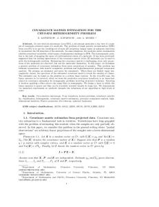
where Tλ (·) : R → R is a thresholding function (Rothman et al., 2009). Some examples of the thresholding function are (i) (hard thresholding) Tλ (s) = I(|s| ≥ λ) · s, (ii) (soft thresholding) Tλ (s) = sign(s) · (|s| − λ)+ , and (iii) (SCAD thresholding) Tλ (s) = I(|s| < 2λ) · sign(s) · (|s| − λ)+ + I(2λ < |s| ≤ aλ) · {(a − 1)s − sign(s)aλ}/(a − 2) + I(|s| > aλ) · s with a > 2. One may threshold only the off-diagonal elements of S, in which case the estimator remains asymptotically equivalent to (3). The universal threshold λ in (3) can be adapted to each element; Cai and Liu (2011) suggests an adaptive thresholding estimator that thresholds each sij with an element-adaptive threshold λij . In section 5, we will use a adaptive thresholding estimator with the soft thresholding function. As we point out earlier, the elementwise manipulation in the thresholding estimators does not retain its PDness. The left panel of Figure 1 plots the minimum eigenvalues of thresholding estimators with various thresholding functions and tuning parameters, when the dataset of n = 100 and p = 400 are sampled from the multivariate t-distribution with 5 degrees of freedom and true covariance matrix M1 defined in Section 4. As shown in the b Thr is not PD if λ is moderately small or selected via the five-fold cross-validation figure, Σ λ (CV) explained in Bickel and Levina (2008a). 5
2.1.2
Banding estimators
The banded covariance matrix arises when the variables of data are ordered and serially dependent as in the data of time series, climatology, or spectroscopy. Bickel and Levina (2008b) proposes a class of banding estimators h i b Band = sij · w|i−j| , Σ h where banding weight wm (m = 0, 1, . . . , p − 1) is proposed by wm = I(m ≤ h) in the b Band discards the sample covariance paper for a fixed bandwidth h. Roughly speaking, Σ h sij if corresponding indices i and j are distant. Cai et al. (2010) considers a tapering b Band as estimator which smooths the banding weight in Σ h when m ≤ h/2 1, wm = 2 − 2m/h, when h/2 < m ≤ h 0, otherwise. We could see that both banding estimators are again from elementwise operations on the sample covariance matrix and, as in the thresholding estimators, do not retain the PDness of the sample estimator. The right panel of Figure 1 tells that this is indeed. The panel is based on the same simulated data set for the left panel and shows that the two estimators result in non-PD estimates regardless of the size of bandwidth.
2.2
Adding PDness to structural (sparse) regularization
The PDness of regularized covariance matrix estimator recently get attention of researchers and a limited number of works are done in the literature; see (Rothman, 2012; Xue et al., 2012; Liu et al., 2014). The three approaches, namely PD sparse estimators, are all based on the fact that the soft thresholding estimator (the thresholding estimator equipped with the soft thresholding function) can be obtained by minimizing the following convex function: h i X b Soft (λ) = (|sij | − λ)+ · sign(sij ) = argmin kΣ − Sk2 + λ Σ |σij |. F Σ
6
i≤j
(4)
Hard thres Soft thres. SCAD thres. 0.0
0.5
1.0
0.5 0.0 −0.5
* *
−1.0
−1.5
*
Min. eigenvalue of banded(tapered) sample cov.
0.5 0.0 −0.5 −1.0
*
−2.0
Min. eigenvalue of thresholded sample cov.
*
Banding Tapering
400
300
Threshold level (lambda)
200
100
0
Bandwidth (h)
Figure 1: Miminum eigenvalues of regularized covariance matrix estimators (n = 100, p = 400). Left for thresholding estimators with threshold (λ) and right for banding estimators with varying bandwidth (h). The star (∗)-marked point is the optimal threshold (bandwidth) selected by a five-fold cross-validation (CV). Note that all the CV-selected estimates are not PD. In each work, a constraint or penalty function is added to (4) to encourage the solution to be PD. For example, Rothman (2012) considers to add a log-determinant penalty: b logdet (λ) := argmin kΣ − Sk2 + τ log det (Σ) + λ Σ F Σ
X
|σij |,
(5)
i 0 is fixed a small value. The additional term behaves a convex barrier that naturally ensures the PDness of the solution and preserves the convexity the objective function. In the paper, the author solves the normal equations with respect to Σ, where column vectors of the current estimate Σ are alternatingly updated by solving (p − 1)variate lasso regressions. We note that, even each lasso regression can be calculated fast, repeating it for every column leads to O(p3 ) flop computations for the entire matrix to be updated. On the other hand, Xue et al. (2012) proposes to solve b EigCon (λ) := argmin kΣ − Sk2 + λ Σ F Σ : Σ��I
X
|σij |.
(6)
i 0 to determine whether Σ b1 < �, otherwise we do not need to update it. Let γ b1 < �. We solve the following minimization problem:
9
minimize µ,α∈R
subject to
�
b b Φ Σ − Σ
µ,α
(8)
αb γ1 + (1 − α)µ ≥ � ; α ∈ [0, 1).
� b to be at least �. In (8), the first constraint enforces the minimum eigenvalue of Φµ,α Σ The second constraint specifies the range of α, intensity of linear shrinkage, where α = 0 corresponds to the complete shrinkage to µI and α = 1 denotes no shrinkage. By the assumption γ b1 < �, the two constraints also imply that µ ≥ � µ ≥
1 α 1 α �− γ b1 > �− � = � 1−α 1−α 1−α 1−α
for any α ∈ [0, 1).
3.2
The choice of α
Let µ ∈ [�, ∞) be fixed. Provided that γ b1 < �, we have γ b1 < � ≤ µ and 1−α ≥
�−γ b1 µ−γ b1
(9)
� b − Σk b from the constraints of (8). Observe that the objective function satisfies kΦµ,α Σ b and then achieves its minimum when (1 − α) touches the lower bound = (1 − α)kµI − Σk in (9). Thus, we have the following lemma. b be given and assume � > γ Lemma 1. Let Σ b1 . Then for any given µ ∈ [�, ∞), the problem (8), with respect to α, is minimized at α∗ := α∗ (µ) =
3.3
µ−� . µ−γ b1
(10)
The choice of µ
By substituting (10) into (8), we have a reduced problem, which depends only on µ, minimize µ : µ>�
� � �−γ b1
b b b ∗
Φµ,α Σ − Σ =
µI − Σ . µ−γ b1
10
(11)
The solution of (11) differs according to how the matrix norm k · k is defined. We consider two most popular matrix norms in below, the spectral norm k · k2 and the (scaled) Frobenius norm k · kF . b is given and � > γ Lemma 2 (Spectral norm). If Σ b1 , then
� �
b b b1
Φµ,α∗ Σ − Σ ≥ � − γ
for all µ ≥ �,
2
o n γ1 . and the minimum of (11) is achieved for any µ ≥ µS := max �, γbp +b 2 Proof. By the definition of the spectral norm,
�−γ b1 �−γ b1
b max |µ − γ bi |
µI − Σ
= µ−γ b1 µ−γ b1 i 2 �−γ b1 = max {|µ − γ bp |, |µ − γ b1 |} . µ−γ b1 Consider ψ2 (t) := max {|t − a|, |t − b|} /(t − a) with a < b, t ∈ (a, ∞). One can easily verify that ψ2 (t) ≡ 1 when µ ≥ (a + b)/2, and ψ2 (t) > 1 when a < t < (a + b)/2. Now substitute t ← µ, a ← γ b1 , and b ← γ bp . Lemma 2 indicates that whenever we take µ such that µ ≥ µS , the spectral-norm distance between the updated and initial estimators is exactly equal to the difference between their smallest eigenvalues. b is given and � > γ b = Lemma 3 (Scaled Frobenius norm). Assume that Σ b1 . If Σ 6 cI for any scalar c, then
� �
b −Σ b b1 )
Φµ,α∗ Σ
≥ (� − γ
sP
p (b γ −γ b )2 Ppi=1 i γi − γ b1 )2 i=1 (b
F
where γ b :=
P
i
for all µ > �,
(12)
γ bi /p. The equality holds if and only if Pp (b γi − γ b1 )2 µ = µF := Pi=1 . p γi − γ b1 ) i=1 (b
In particular,
� �
b b ∗ Φ Σ − Σ b1
µ,α
≤ �−γ F
11
for all µ ≥ µF .
(13)
Proof. We have that v u p
X u �−γ b1 � − γ b
1 t −1 b = p (µ − γ bi )2
µI − Σ µ−γ b1 µ−γ b1 F i=1 sP p b1 ) − (b γi − γ b1 )]2 �−γ b1 i=1 [(µ − γ = √ p (µ − γ b1 )2 v u p X �−γ b1 u = √ t (θti − 1)2 p i=1 P where θ = θ(µ) = (µ − γ b1 )−1 and ti = γ bi − γ b1 . The minimum of h(θ) = pi=1 (θti − 1)2 P P occurs at θ = ( pi=1 t2i )/( pi=1 ti ) (equivalently µ = µF ), and is equal to P p pi=1 (ti − t¯)2 Pp 2 , i=1 ti b 6= cI ensures that Pp ti 6= 0 and Pp t2 6= 0. which proves (12). In addition, that Σ i=1 i i=1 To check (13), observe that each (θti − 1)2 , as a function of µ, is strictly increasing on (µF , ∞) and converges to 1 as µ → ∞. b = The assumption Σ 6 cI implies that the initial estimator should not be trivial. Finally, as a summary of Lemma 2 and 3, we have the following theorem. b and � > 0 Theorem 1 (Distance between the initial and FSPD estimators). Assume Σ are given. Set ( 1 α∗ := α∗ (µ) = 1−
�−b γ1 µ−b γ1
if γ b1 ≥ � ; if γ b1 < �
µ ∈ [µSF , ∞),
where µSF := max {µS , µF } with µS and µF defined in Lemma 2 and 3, respectively. Then � b − Σk b 2 exactly equals to (� − γ 1. kΦµ,α∗ Σ b1 )+ for any µ ; � b − Σk b F is increasing in µ and bounded between 2. kΦµ,α∗ Σ sP p
� � b )2 (b γi − γ
b b ∗ (� − γ b1 ) Ppi=1 ≤ Φ Σ − Σ b1 )+ .
µ,α
≤ (� − γ 2 (b γ − γ b ) F 1 i=1 i b From the theorem, for any µ in [µSF , ∞), the distance between the initial estimator Σ and its FSPD-updated version is less than (�−b γ1 )+ . Indeed, the Monte Carlo experiments 12
� b is robust to the choice of µ. However, in Section 4 show that the empirical risk of Φµ,α∗ Σ µ = µSF would be a preferable choice if one wants to minimize the Frobenius-norm b while maintaining the spectral-norm distance as minimal. We remark distance from Σ that a special case of the proposed FSPD estimator has been discussed by a group of researchers (Section 5.2 in Cai et al. (2014)). In that study, the authors propose to b to Σ b + (� − γ modify the initial estimator Σ b1 )I. This coincides with our FSPD procedure with α = α∗ and µ → ∞.
3.4
Statistical properties of the FSPD estimator
The convergence rate of FSPD estimator to the true Σ is based on the triangle inequality
� �
� �
b b b b
Φ Σ − Σ ≤ Φ Σ − Σ + Σ − Σ
b
≤ (� − γ b1 )+ + Σ − Σ .
(14)
To establish convergence rate for the modified estimator, we need to assume (A1): The smallest eigenvalue of Σ is such that � < γ1 . The assumption (A1) is the same with that assumed in Xue et al. (2012). It means that the cut-point �, determining the PDness of the covariance matrix estimator, is set as smaller than the smallest eigenvalue of the true covariance matrix. For this choice of �, we claim that the convergence rate of the FSPD estimator is at least equivalent to that of the initial estimator in terms of spectral norm. b be any estimator of the true covariance matrix Σ. Suppose � satisfies Theorem 2. Let Σ (A1), α = α∗ and µ ∈ [µSF , ∞), where α∗ and µSF are defined in Theorem 1. Then, we have
� �
b
b
Φµ,α∗ Σ − Σ ≤ 2 Σ − Σ . 2
2
Proof. For � satisfying (A1), we have
b
(� − γ b1 )+ ≤ (γ1 − γ b1 )+ ≤ Σ − Σ . 2
13
(15)
The first inequality in (15) is simply from � ≤ γ1 and the second inequality follows from the Weyl’s perturbation inequality, which states that if A and B are general symmetric matrices, then max{γi (A) − γi (B)} ≤ kA − Bk2 . i
Combining (14) and (15) completes the proof. We remark that the arguments made for Theorem 2 are completely deterministic and there are no assumptions on how the true covariance matrix is structured or on how the estimator is defined. Thus, the convergence rate of FSPD estimator can be easily adapted to any given initial estimator. In terms of spectral norm, Theorem 2 shows that the FSPD estimator has convergence rate at least equivalent to that of the initial estimator, � � b is a consistent or minimax rate-optimal estimator if Σ b is. which implies that Φµ,α∗ Σ Examples include the banding or tapering estimator (Cai et al., 2010), the adaptive block thresholding estimator (Cai and Yuan, 2012), the universal thresholding estimator (Cai and Zhou, 2012), and the adaptive thresholding estimator (Cai and Liu, 2011). To discuss the convergence rate of the FSPD estimator in Frobenius norm, we further assume (A2) :
|b γ − γ1 | pPp 1 = Op (1). γi − γi )2 /p i=1 (b
The assumption (A2) implies that, in the initial estimator, the estimation error of the smallest eigenvalue has the same asymptotic order with the averaged mean-squared error over all eigenvalues. With the additional assumption (A2), we have the following theorem. b be any estimator of the true covariance matrix Σ. Suppose α = Theorem 3. Let Σ α∗ and µ ∈ [µSF , ∞), where α∗ and µSF are defined in Theorem 1. Then, under the assumptions (A1) and (A2), we have
� � � �
b
b
Φµ,α∗ Σ − Σ = 1 + Op (1) · Σ − Σ . F
F
14
Proof. Under the assumptions (A1) and (A2), the inequality (14) shows
� �
b − Σ
Φµ,α∗ Σ
F
b
≤ (� − γ b1 )+ + Σ − Σ F
b
≤ (γ1 − γ b1 )+ + Σ − Σ F v u p
uX
b − Σ γi − γi )2 /p + Σ = Op (1)t (b
F
i=1
≤
�
�
b
1 + Op (1) Σ − Σ
(16)
F
where the last inequality (16) is from Wielandt-Hoffman inequality: for any symmetric A and B, p X (γi (A) − γi (B))2 ≤ p kA − Bk2F . i=1
� �
b −Σ b γ1 )+ can be very conservative. We remark that the inequality Φµ,α∗ Σ
≤ (�−b F
When µ is close to µF , Theorem 1 implies
� �
b −Σ b b1 )+
≈ (� − γ
Φµ,α∗ Σ F
sP
p (b γ −γ b)2 Ppi=1 i , γi − γ b1 )2 i=1 (b
� �Pp P γi − γ b1 )2 γ bi p. Given a fixed sequence of γ γi − γ bi , the term pi=1 (b b)2 i=1 (b
� �
b −Σ b could be considerably smaller than one. In sequel, the Frobenius norm Φµ,α∗ Σ
F
b becomes much smaller than (� − γ b1 )+ , and possible comparable to Σ − Σ . Thus, the where γ b=
Pp
i=1
F
assumption (A2) is only a sufficient condition, and the conclusion of Theorem 3 could be true in much more generality.
3.5
Computation
The proposed FSPD estimator has by itself a great computational advantage over the existing estimators that incorporate both structural regularization and PDness constraint in optimization problem (Rothman, 2012; Xue et al., 2012; Liu et al., 2014). It is primarily because the FSPD procedure is optimization-free and runs eigenvalue decomposition only once. Moreover, in practice, it can be implemented much more quickly without eigenvalue b decomposition. Recall that the FSPD estimator depends on the four functionals of Σ: 15
P −γ b)2 and pi=1 (b γi − γ b1 )2 which in turn can be written in terms of γ bp , P b and V(b γ ) := pi=1 (b γi − γ b)2 . For γ bp and γ b1 , the largest and smallest eigenvalue of γ b1 , γ
γ bp , γ b1 ,
Pp
γi i=1 (b
a symmetric matrix can be independently calculated from the whole spectrum by the Krylov subspace method (see Chapter 7 of Demmel, 1997 or Chapter 10 of Golub and Van Loan, 2012 for examples), which is faster than the usual eigenvalue decomposition of large-scale sparse matrices. Some of these algorithms are implemented using public and commercial software; for example, the built-in MATLAB function eigs(), which is based on Lehoucq and Sorensen, 1996; Sorensen, 1990, or the user-defined MATLAB function eigifp() (Golub and Ye, 2002), which is available online from the authors’ homepage.1 The other functionals are written as γ b =
X
b γ bi /p = tr(Σ)/p
i
V(b γ) =
X
� 2 b 2 )/p − {tr(Σ)/p} b γ bi2 /p − M(b γ )2 = tr(Σ ,
i
and can be evaluated without the computation of the entire spectrum.
4
Simulation study
We numerically compare the finite sample performances of the FSPD estimator and other existing estimators. For the comparison, we use the soft thresholding estimator with universal threshold in (3) as initial regularized estimator. We show that the FSPD estimator induced by the soft thresholding estimator is comparable in performance to the existing PD sparse covariance matrix estimators and is computationally much faster.
4.1
Empirical risk
We generate samples of p-variate random vectors x1 , . . . , xn from (i) multivariate normal distribution or (ii) multivariate t distribution with 5 degrees of freedom. We consider the following matrices as true Σ: 1
During the simulation, we used eigifp() instead of eigs(), as eigs() failed to converge in the smallest eigenvalue computations for some matrices.
16
1. (“Linearly tapered Toeplitz” matrix) [M1 ]ij :=
�
1−
|i−j| 10
� +
(when [A]ij denotes
the (i, j)-th element of A); 2. (“Overlapped block-diagonal” matrix) [M2 ]ij := I(i = j) + 0.4 I (i, j) ∈ (Ik ∪ {ik + � 1}) × (Ik ∪ {ik + 1}) , where the row (column) index {1, 2, . . . , p} is partitioned into K := p/20 subsets, which are non-overlapping and of equal size, and ik denotes the maximum index in Ik . We generate 100 datasets for each of the 36 possible combinations of distribution ∈ {multivariate normal, multivariate-t}, Σ ∈ {M1 , M2 }, n ∈ {100, 200, 400}, and p ∈ {100, 200, 400}. Pn 1 ¯ )(xi − x ¯ )> , We first compute the sample covariance matrix S := n−1 i=1 (xi − x P b Soft (λ∗ ), where the optimal ¯ := n1 ni=1 xi , and the soft thresholding estimator Σ where x threshold λ∗ is chosen from the five-fold cross-validation (CV) introduced in Bickel and � k Levina (2008a). The candidate set of λ is 100 · maxi x ≤ b ≥ α x∼(µ0 ,Σ0 ) � inf P a> x ≥ b ≥ α inf
(17)
y∼(µ1 ,Σ1 )
The solution to (17) does not have a closed-form formula and should be numerically computed. The PDness of the covariance matrices Σ0 and Σ1 (or their estimators) is a necessary condition for both the convexity of the problem and the existence of a convergent algorithm to the solution. In practice, the true µs and Σs are unknown and we must plug their estimators into the LMPM formulation (17). Lanckriet et al. (2002) uses sample mean and covariance matrices when they are well defined. In case the sample covariance matrix S is singular, they suggest using S + δI with a given constant δ rather than S. 21
5.1.2
Example: Speech recognition
We illustrate the performance of the LMPM with various PD covariance matrix estimators using voice data (Tsanas et al., 2014)2 . The dataset comprises 126 signals representing the pronunciation of vowel /a/ by patients with Parkinson’s disease. Each signal was preprocessed into 309 features and labeled as “acceptable” or “unacceptable” by an expert. The dataset is in the form of a 126 × 309 matrix with binary labels. In order to measure classification accuracy, we randomly split the dataset 100 times into 90% training samples and 10% testing samples; the LMPM is constructed using the training samples and classification accuracy is measured using the testing samples. In building the LMPM, the true mean vectors are estimated from the sample means and covariance matrices are estimated from the following PD estimators: (1) “Sample,” the sample covariance matrix added by δI, where δ = 10−2 ; (2) “Diagsample,” the diagonal matrix of the sample variances; (3) “LedoitWolf,” the linear shrinkage estimator by Ledoit and Wolf (2004); (4) “CondReg,” the condition-number-regularized estimator by Won et al. (2013); (5) “Adap.+EigCon,” the eigenvalue constraint estimator by Xue et al. (2012) based on the adaptive thresholding estimator by Cai and Liu (2011); and (6) “Adap.+FSPD,” the proposed FSPD estimate (α = α∗ , µ = µSF ) induced by the adaptive thresholding estimator. Here, unlike the numerical study in Section 4, we use the adaptive thresholding estimator as an initial regularized covariance estimator instead of the (universal) soft thresholding estimator. This is because marginal variances of the given data can be unequal over variables, in which case adaptive thresholding is known to perform better than the universal thresholding (Cai and Liu, 2011). The tuning parameter of the adaptive thresholding estimator is selected using five-fold CV as in Cai and Liu (2011). The pre-determined constant � for Adap.+EigCon and Adap.+FSPD is set as 10−2 . The average and standard deviation of classification accuracy over 100 random par2
The data are available on the UCI Machine Learning Repository (http://archive.ics.uci.edu/ ml/).
22
titions are reported in Table 5. All the regularization methods (items 3–6) show better classification accuracy than the naive sample covariance matrix (item 1). In addition, Adap.+FSPD has the highest accuracy with average 89.2% and standard deviation 9.2%. This record is highly competitive to the results reported in the original paper (Tsanas et al., 2014), which is based on a random forest and support vector machine after a feature selection algorithm named LOGO by Sun et al. (2010). Finally, we note that the entire process of Adap.+FSPD, from covariance matrix estimation to LMPM construction, takes only 0.68 seconds. Sample 73.8 (12.4)
Diagsample 76.4 (12.6)
LedoitWolf 86.9 (10.7)
CondReg 75.3 (13.6)
Adap.+EigCon 82.0 (18.1)
Adap.+LSPD 89.2 (9.2)
Table 5: The average classification accuracies (standard deviations in parenthesis) for the LMPM with selected PD covariance matrix estimators based on 100 random partitions. The abbreviations of the estimators are introduced in the main body of the section.
5.2 5.2.1
Markowitz portfolio optimization Minimum-variance portfolio allocation and short-sale
In finance, portfolio refers to a family of (risky) assets held by an institution or private individual. If there are multiple assets to invest in, a combination of assets is considered and it becomes an important issue to select an optimal allocation of portfolio. Minimum variance portfolio (MVP) optimization is one of the well-established strategies for portfolio allocation (Chan, 1999). The author proposes to choose a portfolio that minimizes risk, standard deviation of return. Since the MVP problem may yield an optimal allocation with short-sale or leverage, Jagannathan and Ma (2003) proposes to add a no-short-sale constraint to the MVP optimization formula. We introduce the two approaches briefly. Let r := (r1 , . . . , rp )> be a p-variate random vector in which each rj represents the return of the j-th asset constituting portfolio (j = 1, . . . , p). Denote by Σ := Var(r) the unknown covariance matrix of assets. A p-by-1 vector w represents an allocation of the investor’s wealth in such a way that each
23
wj stands for the weight of the j-th asset and
Pp
j=1
wj = 1. Then, the MVP optimization
by Chan (1999) is formulated as minimize w> Σw subject to w> 1 = 1. w
(18)
Note that (18) allows its solution to have a weight that is negative (short-sale) or greater than 1 (leverage). Jagannathan and Ma (2003) points out that short-sale and leveraging are sometimes impractical because of legal constraints and considers the MVP optimization problem with no short-sale constraint: minimize w> Σw subject to w> 1 = 1, w ≥ 0, w
(19)
where w ≥ 0 is defined component-wise. The combination of two constraints in (19) ensures that the resulting optimal weights are restricted to [0, 1]. Jagannathan and Ma (2003) empirically and analytically illustrate that (19) could have a smaller risk than (18) even if the no-short-sale constraint is wrong. We note that the paper handles only the case in which the sample covariance matrix is nonsingular and plugged into the unknown Σ in (19). In principle, Σ can be replaced by a suitable PD estimator. 5.2.2
Example: Dow Jones stock return
The aim of this analysis is not only to reproduce with different data the finding of Jagannathan and Ma (2003) that the no-short-sale constraint does not affect the risk of (18), but also to investigate empirically whether the same conclusion can hold for another choice of PD covariance matrix estimator. We compare two portfolio optimization schemes: simple MVP (18) and no-short-sale MVP (19). The unknown covariance matrix Σ is estimated with seven PD covariance matrix estimators. Five estimators, (1) “Sample,” (2) “LedoitWolf,” (3) “CondReg,” (4) “Adap.+EigCon,” and (5) “Adap.+FSPD,” are already introduced in Section 5.1.2. To these, we add (6) “POET+EigCon,” an eigenvalue constraint estimator based on the POET estimator proposed by Fan et al. (2013) (see Xue et al. (2012)’s discussion section in the cited paper), and (7) “POET+FSPD,” the FSPD estimator induced by the POET estimator. The reason why we additionally 24
consider (6) and (7) is that stock return data are believed to have a factor structure that can supposedly be reflected through the POET estimation. As data, we use the 30 stocks that constituted the Dow Jones Industrial Average in July 2008; previously, these were used in Won et al. (2013). The dataset contains the daily closing prices from December 1992 to June 2008, adjusting for splits and dividend distributions. The portfolios are constructed as follows. For covariance matrix estimation, we use the stock returns of the past 60 or 240 trading days (approximately 3 or 12 months, respectively). As Condreg, Adap, and POET require the selection of tuning parameters, they are done via five-fold CV in which the returns of each day are treated as independent samples. Once the portfolios are established by solving (18) and (19) with covariance matrices plugged in by the corresponding estimators, we hold each for 60 trading days. This process begins on February 18, 1994, and is continually repeated until July 6, 2008, producing 60 holding periods in total. We record all the returns for each trading day and summarize them in the form of realized return, realized risk, and the Sharpe ratio. Here, the realized return and realized risk of a portfolio are defined as the average and standard deviation of daily returns from that portfolio, respectively. The Sharpe ratio is a risk-adjusted performance index, defined as {(realized return) - (risk-free rate)}/(realized risk). The risk-free rate is set at 5% per annum. We present some interpretations and conjectures based on the results summarized in Table 6. We first compare the realized risks of the simple and no-short-sale MVPs; the third and fourth columns of the table show that the differences in the realized risks of the respective MVPs are competitive. The sample covariance matrix reproduces the findings of Jagannathan and Ma (2003), that is, that no-short-sale MVPs have a smaller risk than simple MVPs. In addition, we find that the regularized covariance matrix estimators (LedoitWolf, Condreg, the two Adap.s, and the two POETs) also produce similar results. Interestingly, the results of realized returns in the first and second columns show that no-short-sale MVPs produce higher realized returns than all simple MVPs except for Condreg, showing a relative improvement of the Sharpe ratios in all cases except for 25
Realized return [%] Realized risk [%] Sharpe Ratio Simple No Short. Simple No Short. Simple No Short. (Portfolio rebalancing based on 60 previous trading days) Sample 22.49 23.11 3.28 3.34 5.33 5.41 LedoitWolf 21.25 21.61 3.11 3.06 5.23 5.44 CondReg 24.70 24.70 4.17 4.16 4.73 4.73 Adap.+FSPD 22.74 23.26 3.59 3.62 4.95 5.04 Adap.+EigCon 22.74 23.38 3.35 3.40 5.30 5.40 20.99 21.85 3.13 3.07 5.11 5.49 POET+FSPD POET+EigCon 20.81 21.28 3.18 3.06 4.96 5.32 (Portfolio rebalancing based on 240 previous trading days) 22.42 23.07 3.33 3.37 5.24 5.36 Sample LedoitWolf 21.72 23.08 2.89 2.94 5.78 6.14 24.91 24.73 4.18 4.18 4.76 4.72 CondReg Adap.+FSPD 22.68 23.13 3.57 3.60 4.95 5.04 22.47 3.30 3.36 4.92 5.19 Adap.+EigCon 21.25 POET+FSPD 21.49 23.94 3.02 2.98 5.46 6.35 POET+EigCon 20.93 23.49 3.07 2.99 5.18 6.19 Table 6: Empirical out-of-sample performances, from 30 constituents of DJIA with 60 days of holding, starting from 2/18/1994. All the rates are annualized.
Condreg. Next, we compare the 60- and 240-day training results for the construction of portfolios (rows 1–6 and 7–12). Unlike the Sample and the Adap.s, both LedoitWolf and the POETs show higher realized returns and Sharpe ratios for the 240-day training. This is true for both simple and no-short-sale MVPs. We conjecture that the factored structure of the POET estimation captures the latent structures of stocks better in long-history data than short-history data. However, the higher weight on the identity matrix in LedoitWolf made the portfolio behave as an equal-weight investment strategy, which is practically known to work well in long-term investment. Condreg performs somewhat differently from other regularized covariance matrix estimators; the realized return of Condreg dominates those of the other methods. This confirms the results in Won et al. (2013), which illustrates that an MVP with Condreg produces the highest wealth growth. This seems to be empirical evidence for “high risk, high return,” as CondReg shows the highest realized risk.
26
Finally, we compare the two PD covariance matrix estimation methods, that is, the FSPD estimators (Adap.+LSPD and POET+FSPD) and the eigenvalue constraint estimators (Adap.+EigCon and POET+EigCon). For POET-based estimation, FSPD approaches produce higher Sharpe ratios than the eigenvalue constraint methods in all cases. For adaptive thresholding estimation, eigenvalue constraint methods have higher Sharpe ratios than the FSPD estimates except for the case of a simple MVP applied for over 60 trading days. However, the POET+FSPD approach applied for over 240-trading days produces the highest Sharp ratios for MVPs for both the simple and no-short-sale cases. In addition, as the FSPD estimators are far simpler and faster than the eigenvalue constraint estimator, they are more desirable for practical use.
6
Estimation of positive definite precision matrices
In this section, we emphasize that the FSPD approach can be applied to estimating PD precision matrix estimators as well. Let Ω = Σ−1 be the unknown true precision matrix b be one of its estimators, which possibly lacks PD. In the theory presented in and Ω b can be treated as a generic symmetric matrix and thus Section 3, the initial estimator Σ b Therefore, we have the following theorem. Theorem 1 is valid for Ω. b be any estimator of the true precision matrix Ω. Suppose α = α∗ Theorem 4. Let Ω and µ ∈ [µSF , ∞), where α∗ and µSF are defined in Theorem 1 with γ bi , being understood b Then, under the assumption (A1), we have by the i-th smallest eigenvalue of Ω.
� �
b
b
Φµ,α∗ Ω − Ω ≤ 2 Ω − Ω . 2
2
Further, if (A2) holds additionally,
� � � �
b
b − Ω − Ω .
Φµ,α∗ Ω
= 1 + Op (1) · Ω F
F
Theorem 4 implies that, as in the estimation of the PD covariance matrix, the FSPDupdated precision matrix estimator can preserve both the support and convergence rate. Several regularization methods are proposed for sparse precision matrices, and, like regularized covariance matrix estimation, these proposed estimators do not guarantee 27
PDness in finite sample. Examples include CLIME by Cai et al. (2011), neighborhood selection by Meinshausen and B¨ uhlmann (2006), SPACE by Peng et al. (2009), symmetric lasso by Friedman et al. (2010), and CONCORD by Khare et al. (2015). In addition, penalized Gaussian likelihood methods, whose very definition ensures PDness of the solution, may have a solution lacking PDness, since the relevant optimization algorithms approximate solutions by a non-PD matrix. For instance, Mazumder and Hastie (2012) reports that the graphical lasso algorithm by (Friedman et al., 2008; Witten et al., 2011) solves the problem in an indirect way and could return non-PD solutions. Despite the possibility of non-PDness, we empirically find that the precision matrix estimators listed above are likely to be PD; thus, they suffer minimally from potential b non-PDness. Let Ω(λ) be a regularized precision estimator with tuning parameter λ. b b Although non-PDness often arises in Ω(λ) when λ is not large and Ω(λ) is dense, we b ∗ ) is PD in most cases. The observe that, with optimal selection of λ∗ through CV, Ω(λ case Ω = M1 (tapered Toeplitz matrix) is the only one in which we find non-PDness in some precision matrix estimators (CONCORD and symmetric lasso). Table 6 summarizes the spectral information of these estimators. p 100 200 400
N t N t N t
CONCORD Min. eig. 2.49e-03 (2.44e-05) 2.12e-03 (4.07e-05) 5.90e-04 (1.03e-05) 3.05e-04 (2.41e-05) -3.44e-04 (4.09e-05) -3.43e-04 (1.21e-04)
#(PD) 100/100 100/100 100/100 92/100 14/100 23/100
Symmetric lasso Min. eig. #(PD) 2.55e-03 (2.66e-05) 100/100 2.23e-03 (4.89e-05) 100/100 6.55e-04 (1.03e-05) 100/100 4.11e-04 (2.33e-05) 94/100 -1.60e-04 (1.00e-07) 4/100 -2.92e-04 (2.80e-05) 9/100
Table 7: Spectral information of selected sparse precision matrix estimators when the true precision matrix is M1 (tapered Toeplitz matrix).
7
Concluding remarks
In this study, we propose a two-stage approach with covariance matrix regularization and the conversion toward PDness considered to be two separate steps. Because of its 28
two-staged nature, the proposed FSPD procedure can be combined with any regularized covariance or precision matrix estimator. The procedure considers a convex combination involving only the initial regularized estimator and the related parameters can be selected in explicit form. Thus, the FSPD procedure is optimization-free and can be quickly computed. Despite its simplicity, the FSPD estimator enjoys theoretical advantages, in that it can preserve both the sparse structure and convergence rate of a given initial estimator. The FSPD procedure finds a PD matrix close to the initial estimator subject to the class of linear shrinkage estimators. Here, we conclude the paper with a discussion on the linear shrinkage constraint in the FSPD. Consider three classes of covariance matrices b∗ : Σ b ∗ = (Σ b ∗ )> , γ1 (Σ b ∗ ) ≥ �}, S1 = {Σ b ∗ ∈ S0 : supp(Σ b ∗ ) = supp(Σ)}, b S0 = {Σ and b ∗ ∈ S0 : Σ b ∗ = αΣ b + (1 − α)µI, α ∈ [0, 1], µ ∈ R}. In (1), we originally aim to S2 = {Σ b ∗ − Σk b given Σ. b However, in (2), we solve min b ∗ kΣ b ∗ − Σk b (FSPD) solve minΣb ∗ ∈S1 kΣ Σ ∈S2 instead of (1), because its solution can be written explicitly. It would be of interest to know the cost of solving (2) instead of (1)—to be specific, the difference between b ∗ − Σk b and min b ∗ kΣ b ∗ − Σk. b minΣb ∗ ∈S2 kΣ Σ ∈S1 First, we find no cost in view of the spectral norm. Suppose that γ b1 and γ b1∗ are the b and Σ b ∗ , respectively. We know that kΣ b ∗ − Σk b 2≥γ b1 ≥ minimum eigenvalues of Σ b1∗ − γ b ∗ ∈ S0 , and thus min b ∗ kΣ b ∗ − Σk b 2 ≥ �−γ �−γ b1 for all Σ b1 . Recall that Lemma 2 Σ ∈S0 b ∗ − Σk b 2 ≤ � − γ1 , and implies that minΣb ∗ ∈S2 kΣ b ∗ − Σk b 2 ≤ min kΣ b ∗ − Σk b 2 ≤ min kΣ b ∗ − Σk b 2 ≤ � − γ1 min kΣ
b ∗ ∈S0 Σ
b ∗ ∈S1 Σ
b ∗ ∈S2 Σ
b ∗ − Σk b 2 = min b ∗ kΣ b ∗ − Σk b 2 =�−γ because S2 ⊆ S1 ⊆ S0 . Therefore, minΣb ∗ ∈S2 kΣ b1 . Σ ∈S1 Thus, no additional cost is given by using the linear shrinkage constraint in spectral norm. b∗ − Second, in view of the Frobenius norm, we recall that Lemma 3 tells minΣb ∗ ∈S2 kΣ rP p p (b γ −b γ )2 b ∗ −Σk b F = Pp (� − γ b F = (�−b bi )2+ /p. Σk γ1 )· Ppi=1(bγii−bγ1 )2 , whereas, in general, minΣb ∗ ∈S0 kΣ i=1 i=1
The two bounds (minimums) depend on the eigenvalues of the true covariance matrix and the initial estimator in a complex way and hard to understand their closeness. For example, suppose we consider the FSPD estimator based on the soft thresholding estimator. 29
A numerical investigation, not reported in this paper, shows the difference between two bounds decreases as p increases in all the scenarios of Σ = M2 in Section 4. However, we do not find any special pattern in the scenarios of Σ = M1 .
References Bai, Z. and Silverstein, J.W. (2010). Spectral Analysis of Large Dimensional Random Matrices, Springer, New York. Bickel, P. and Levina, E. (2008a). Covariance regularization by thresholding. The Annals of Statistics, 36(6), 2577–2604. Bickel, P. and Levina, E. (2008b). Regularized estimation of large covariance matrices. The Annals of Statistics, 36(1), 199–227. Bien, J. and Tibshirani, R. (2011). Sparse estimation of a covariance matrix. Biometrika, 98(4), 807–820. Boyd, S., Parikh, N., Chu, E., Peleato, B., and Eckstein, J. (2010). Distributed optimization and statistical learning via the alternating direction method of multipliers. Foundations and Trends in Machine Learning, 3(1), 1-122. Cai, T. and Liu, W. (2011). Adaptive thresholding for sparse covariance matrix estimation. Journal of the American Statistical Association, 106(494), 672–684. Cai, T., Liu, W., and Luo, X. (2011). A constrained `1 minimization approach to sparse precision matrix estimation. Journal of the American Statistical Association, 106(494), 594–607. Cai, T. and Low, M. (2015). A framework for estimation of convex functions. Statistica Sinica, 25, 423-456.
30
Cai, T., Ren, Z., and Zhou, H. (2014). Estimating structured high dimensional covariance and precision matrices: Optimal rates and adaptive estimation. Technical report available from http://www-stat.wharton.upenn.edu/~tcai/. Cai, T. and Yuan, M. (2012). Adaptive covariance matrix estimation through block thresholding. The Annals of Statistics, 40(4), 2014–2042. Cai, T., Zhang, C.H., and Zhou, H. (2010). Optimal rates of convergence for covariance matrix estimation. The Annals of Statistics, 38(4), 2118–2144. Cai, T.. and Zhou, H. (2012). Optimal rates of convergence for sparse covariance matrix estimation. The Annals of Statistics, 40(5), 2389–2420. Chan, L. (1999). On portfolio optimization: Forecasting covariances and choosing the risk model. Review of Financial Studies, 12(5), 937–974. Demmel, J.W. (1997). Applied Numerical Linear Algebra. SIAM, Philadelphia, PA. Fan, J., Liao, Y., and Mincheva, M. (2013). Large covariance estimation by thresholding principal orthogonal complements. Journal of the Royal Statistical Society: Series B, 75(4), 603–680. Friedman, J., Hastie, T., and Tibshirani, R. (2008). Sparse inverse covariance estimation with the graphical lasso. Biostatistics, 9(3), 432–441. Friedman, J., Hastie, T., and Tibshirani, R. (2010). Applications of the lasso and grouped lasso to the estimation of sparse graphical models. Technical report, Stanford University, Stanford, CA. Golub, G.H. and Van Loan, C. F. (2012). Matrix Computations (4th edition). Johns Hopkins University Press, Baltimore. Golub, G.H. and Ye, Q. (2002). An inverse free preconditioned Krylov subspace method for symmetric generalized eigenvalue problems. SIAM Journal on Scientific Computing, 24(1), 312?334. 31
Green, R. C. and Hollifield, B. (1992). When will mean-variance efficient portfolios be well diversified? The Journal of Finance, 47(5), 1785–1809. Jagannathan, R. and Ma, T. (2003). Risk reduction in large portfolios: Why imposing the wrong constraints helps. The Journal of Finance, 58(4),1651–1683. Khare, K., Oh, S.-Y., and Rajaratnam, B. (2015). A convex pseudolikelihood framework for high dimensional partial correlation estimation with convergence guarantees. Journal of the Royal Statistical Society: Series B, To appear. Lam, C. and Fan, J. (2009). Sparsistency and rates of convergence in large covariance matrix estimation. The Annals of Statistics, 37(6B), 4254–4278. Lanckriet, G., El Ghaoui, L., Bhattacharyya, C., and Jordan, M.I. (2002). A robust minimax approach to classification. The Journal of Machine Learning Research, 3, 555–582. Ledoit, O. and Wolf, M. (2004). A well-conditioned estimator for large-dimensional covariance matrices. Journal of Multivariate Analysis, 88(2), 365–411. Lehoucq, R. and Sorensen, D. (1996). Deflation techniques for an implicitly restarted Arnoldi iteration. SIAM Journal on Matrix Analysis and Applications, 17(4), 789– 821. Liu, H., Wang, L., and Zhao, T. (2014). Sparse covariance matrix estimation with eigenvalue constraints. Journal of Computational and Graphical Statistics, 23(2), 439–459. Luenberger, D.G. (2013). Investment Science (2nd edition). Oxford University Press, New York. Marcenko, V. and Pastur, L. (1967). Distribution of eigenvalues for some sets of random matrices. Mathematics of the USSR-Sbornik, 1(4), 457–483. Markowitz, H. (1952). Portfolio selection. The Journal of Finance, 7(1), 77–91. 32
Mazumder, R. and Hastie, T. (2012). The graphical lasso: New insights and alternatives. Electronic Journal of Statistics, 6, 2125–2149. Meinshausen, N. and B¨ uhlmann, P. (2006). High-dimensional graphs and variable selection with the Lasso. The Annals of Statistics, 34(3), 1436–1462. Merton, R.C. (1980). On estimating the expected return on the market. Journal of Financial Economics, 8, 323–361. Peng, J., Wang, P., Zhou, N., and Zhu, J. (2009). Partial correlation estimation by joint sparse regression models. Journal of the American Statistical Association, 104(486), 735–746. Rothman, A. J. (2012).
Positive definite estimators of large covariance matrices.
Biometrika, 99(3), 733–740. Rothman, A., Levina, E., and Zhu, J. (2009). Generalized thresholding of large covariance matrices. Journal of the American Statistical Association, 104(485), 177–186. Sorensen, D. (1990). Implicit application of polynomial filters in a k-step Arnoldi method. SIAM Journal on Matrix Analysis and Applications, 13(1):357–385. Stein, C. (1956). Inadmissibility of the usual estimator for the mean of a multivariate normal distribution. In Proc. Third Berkeley Symp. on Math. Statist. and Prob., 1, 197–206. Sun, Y., Todorovic, S., and Goodison, S. (2010). Local learning based feature selection for high dimensional data analysis. IEEE Transactions on Pattern Analysis and Machine Intelligence, 32(9), 610–626. Tsanas, A., Little, M., Fox, C., and Ramig, L. O. (2014). Objective automatic assessment of rehabilitative speech treatment in Parkinson’s disease. IEEE Transactions on Neural Systems and Rehabilitation Engineering, 22(1):181–190.
33
Witten, D., Friedman, J., and Simon, N. (2011). New insights and faster computations for the graphical lasso. Journal of Computational and Graphical Statistics, 20(4), 892–900. Won, J-H., Lim, J., Kim, S-J., and Rajaratnam, B. (2013). Condition number regularized covariance estimation. Journal of the Royal Statistical Society. Series B, 75(3), 427– 450. Xue, L., Ma, S., and Zou, H. (2012). Positive-definite `1 -penalized estimation of large covariance matrices. Journal of the American Statistical Association, 107(500),1480– 1491.
34