392
JOURNAL OF ATMOSPHERIC AND OCEANIC TECHNOLOGY
VOLUME 20
An Adjoint Ocean Model Using Finite Elements: An Application to the South Atlantic UWE DOBRINDT Alfred Wegener Institute for Polar and Marine Research, Bremerhaven, and STN Atlas Elektronik GmbH, Bremen, Germany
JENS SCHRO¨TER Alfred Wegener Institute for Polar and Marine Research, Bremerhaven, Germany (Manuscript received 14 September 2000, in final form 13 June 2002) ABSTRACT A new inverse model to study the large-scale ocean circulation and its associated heat and freshwater budget is developed. The model relies on traditional assumptions of mass, heat, and salt conservation. A three-dimensional velocity field that is in steady state and obeys geostrophy is derived. Using this flow field, the steadystate advection–diffusion equations for temperature and salinity are solved and the corresponding density is calculated. An optimization approach is used that adjusts reference velocities to get model parameters close to observations so that the velocities are in geostrophic balance with the model density field. In order to allow a variable spatial resolution, the finite-element method is used. The mesh is totally unstructured and the threedimensional elements are tetrahedra. Climatological hydrographic data, observations of sea surface height (SSH) from satellite altimetry, and wind data are assimilated in the model. The advantages of the finite-element method make it possible to use an easy representation of the model parameters on the tetrahedra. It is not difficult to find the adjoint form of the discrete equations. The unstructured mesh agrees well with the complex geometry of the bottom topography. The model is applied to the South Atlantic. First model results show that the upperlevel circulation corresponds to the circulation known from literature. The volume transport through Drake Passage is constrained to be 130 Sv. The transports of water masses, heat, and salt across the open boundaries (Drake Passage, 308S, 208E) are in agreement with the literature. The formation rate of bottom water is 13.0 Sv and the heat transport across 308S to the north is 0.64 PW.
1. Introduction Describing the global ocean circulation is still a problem despite more than 100 years of systematic observation and research in oceanography. The large-scale transport and the distribution of water masses can be derived from hydrographic data (temperature and salinity) using the geostrophic equations. The hydrographic datasets are spatially and temporally inhomogeneous and geostrophy can be used only to describe the vertical shear of the velocity field. To get absolute velocities it is often assumed that the flow velocity vanishes at some reference depth. The error made by this assumption is small near the surface where the velocities are larger than in the deep ocean where they have an order of 0.01 m s 21 . As a consequence a small shift of the reference level can produce errors of the latter order of magnitude. In local regions where the ocean is shallower than the reference depth the bottom depth has to be chosen as reference, for example. Corresponding author address: Dr. Uwe Dobrindt, STN Atlas Elektronik GmbH, Sebaldsbru¨cker Heerstr. 235, 28305 Bremen, Germany. E-mail:
[email protected]
q 2003 American Meteorological Society
Another possibility to calculate absolute velocities is the determination of reference velocities at the ocean surface. The velocities in the deep ocean can be calculated by vertical integration from the surface. As a second independent dataset, measurements from satellite altimetry can be used to determine the reference velocities. Numerical models and assimilation techniques are combined for this purpose. The model states computed must fulfill the model equations and have to take into account the data. Strictly speaking, data assimilation is used for prognostic models. Diagnostic models where the model parameters are adapted to the data are called inverse models. An optimization approach is applied to fit the parameters. A so-called cost function is minimized subject to the model equality constraints. Basic concepts are described by Thacker (1988), Olbers (1989), and Wunsch (1996). Computations with this method were made, for example, by Schro¨ter (1989). Schro¨ter et al. (1993) and Vogeler and Schro¨ter (1995, 1999) applied the method to regional eddy-resolving ocean models. Schlitzer (1993, 1995) developed a box model for the Atlantic, which is extended to the global ocean (de las Heras and Schlitzer 1999). Nechaev and
MARCH 2003
¨ TER DOBRINDT AND SCHRO
Yaremchuk (1995) and Yaremchuk et al. (1998) presented an adjoint model for analyzing hydrographic sections. A global model to investigate the barotropic ocean circulation originated from Seiß (1996). Sloyan (1997) presented a box model for the Southern Ocean. The models mentioned above are box models and/or use the finite-difference method (FDM). In the present model the finite-element method (FEM) is used. Originally the FEM was developed in the 1950s and 1960s to solve problems occuring in elastomechanics. Later the FEM was expanded for applications to many other physical processes that are described by partial differential equations. The theory of the FEM is described in detail, for example, by Zienkiewicz (1977) and Johnson (1990). There are successful applications in tidal models since the beginning of the 1970s. Examples are the works of Connor and Wang (1973), Walters and Werner (1989), and Le Provost and Vincent (1991). But there are only a few works that use the FEM in (global) circulation models. A first work was presented by Fix (1975) with a quasigeostrophic model. Haidvogel et al. (1980) compared the FEM with the FDM. For problems in fluid dynamics and particularly for convection–and advection–diffusion problems the FEM became popular in the 1980s. At that time different upwind methods for stabilization were developed. A basic work is given by Brooks and Hughes (1982). In recent years Myers and Weaver (1995) used the FEM in a diagnostic barotropic ocean model. Iskandarani et al. (1995) presented a spectral finite-element model for the shallow water equations. With a similar model Haidvogel et al. (1997) described the global circulation and Wunsch et al. (1997) investigated the dynamics of long-period tides. This model was also used by Taylor et al. (1997), Levin et al. (1997), and Curchitser et al. (1998, 1999). Further developments of finite-element models for the shallow water equations were presented by Behrens (1996, 1998), Le Roux et al. (1998), and Giraldo (1999, 2000a,b). Zhu et al. (1994) worked with data assimilation in a two-dimensional finite-element model for the shallow water equations. Another finite-element circulation model is QUODDY (Ip and Lynch 1995), which is used for regional comprehensive coastal modeling (Lynch et al. 1996). QUODDY is based on the conventional three-dimensional shallow water equations. It is tide resolving to investigate shelf circulation. The meshes are created by prisms and a general terrain-following vertical coordinate is used. Recently, an inverse model version of QUODDY has been designed that uses an assimilation scheme such as the adjoint method (Lynch and Hannah 2001). Altogether applications of the FEM in oceanography—especially in three-dimensional inverse models—are still rare. The major goal of this work is the development of an internally consistent three-dimensional adjoint model using finite elements to investigate the large-scale ocean circulation. The model solves the stationary advection–
393
diffusion problem. A mesh is generated with tetrahedra. These elements are particularly suitable to represent the complex three-dimensional geometry given by the bottom topography. The mesh is totally unstructured so that any local refinement is possible. This is one of the great advantages of the FEM compared to the FDM. Another advantage is that the adjoint code can be created relatively easily. The model describes a flow field in geostrophic balance and conserves mass and heat. The control variables of the inverse model are horizontal reference velocities at the ocean surface and sources (heat and freshwater fluxes) in the advection–diffusion equation. Assimilated data are among others climatologic hydrographic data and sea surface height (SSH) data from satellite altimetry. The second major goal of this work is a first application of the model to the South Atlantic to study the large-scale circulation, the formation and spreading rates of water masses and the exchange of heat and salt. The investigations focus on the Weddell Sea. The organization of this paper is as follows: the governing model equations and the strategy of the adjoint model are described in section 2. In section 3 the use of the FEM is presented. The application of the model and its results are discussed in sections 4 and 5. Finally, a summary and conclusions are given in section 6. 2. The inverse model In this section the strategy of the model is presented. The model parameters are temperature T, salinity S, density r, velocities u 5 (u h , w) 5 (u, y , w), and sources F T and F S of the advection–diffusion equation for temperature and salinity. The density r is calculated from the temperature field and the salinity field with the equation of state. Using the density and a prescribed reference velocity the horizontal flow field u h is computed and from that the vertical velocities w are determined using volume conservation. Solving the advection–diffusion equations with this flow field yields new temperatures and salinities. Data are assimilated with the adjoint method in the model. A cost function J fits the model to the data and measures the quality of the model solution. The model parameters are divided into independent parameters—the control variables of the cost function—and into dependent parameters. We solve for a set of parameters that minimize the value of the cost function. This set represents a certain circulation pattern (flow field) and the corresponding temperature and salinity fields that are both in geostrophic and advective– diffusive balance. a. Model equations The general ocean circulation is described by equations of motion that are modified Navier–Stokes equations including the effects of the rotating earth. The fluid
394
JOURNAL OF ATMOSPHERIC AND OCEANIC TECHNOLOGY
VOLUME 20
is only a thin stratified layer on the earth sphere. This is taken into consideration by certain approximations. A detailed treatment and the concepts of this subject are given in the book of Gill (1982), for example. The surface circulation is mainly wind driven but the deep circulation is determined by the gradients of pressure and density, respectively. The density r depends on the temperature T and the salinity S of the seawater and is given by a highly nonlinear equation of state:
The advective transport and the diffusion of the thermodynamic tracers temperature and salinity is given by the stationary advection–diffusion equation
E r 5 r 2 R(T, S, p) 5 0,
Here K h and K y are the horizontal and the vertical diffusion coefficients. The sources F T and F S are implemented to parameterize subscale processes, which are not resolved by the model because of its properties (e.g., local grid spacing). Using this set of model equations to determine the deep circulation for a steady state is a common choice for inverse models (see Wunsch 1996). The independent model parameters (control variables) are the horizontal reference velocities uref and y ref and the sources F T and F S :
(1)
where p 5 0.1Dz is the pressure in bars. A formula (socalled UNESCO formula 1981) for R is presented by Gill (1982). For a small ratio between the nonlinear term and the Coriolis force in the equations of motion and a small aspect ratio (ratio between the characteristic depth and the characteristic length of the ocean) the horizontal flow field is described, to lowest order, by the geostrophic equations: fy 5
1 ]p , r ]x
fu 5 2
1 ]p . r ]y
(2)
There u and y are the horizontal velocities, g is the acceleration of gravity and f 5 2V sinf is the Coriolis parameter. The geostrophic approximation represents the balance between the Coriolis force and the pressure gradient. Together with the hydrostatic balance ]p/]z 5 2gr the thermal wind relation ]u g ]r 5 , ]z r f ]y
]y g ]r 52 , ]z r f ]x
(3)
can be derived, which yields only the vertical shear of the flow field. On the other hand, the unknown pressure field of the geostrophic relation is now replaced by the density field, which can be measured. Vertical integration of the thermal wind equations with reference to the spatially varying velocities uref and y ref at the surface results in E u 5 u(x, y, z) 2 uref (x, y) 1 E y 5 y (x, y, z) 2 y ref (x, y) 2
g rf g rf
E E
2h e
]r dz9 5 0, ]y
2h e
]r dz9 5 0. ]x (4)
z
z
In the Ekman layer (0 $ z $ 2h e ) u h (z) 5 uref 5 (uref , y ref ) is valid. The vertical velocities are computed by vertical integration of the equation of continuity. The integration begins at the bottom with the kinematic boundary condition w(2H) 5 u h · =H and ends at the depth 2h e of the Ekman layer: E w 5 w(z) 1
E
z
2H
5 w(z) 1 = ·
1
1E
2
2H
2
u h dz9 5 0.
]2 T 2 F T 5 0, ]z 2
E S 5 u · =S 2 K h D h S 2 Ky
]2 S 2 F S 5 0. ]z 2
(6)
p 5 [. . . , uref, j , . . . , y ref, j , . . . , F Tj , . . . , F Sj , . . .]T .
(7) The other horizontal velocities and the temperature T, the salinity S, the density r, and the vertical velocities w constitute the set of dependent parameters q 5 [. . . , u i , . . . , y i , . . . , Ti , . . . , S i , . . . ,
r i , . . . , w i , . . .]T .
(8)
The control variables p are initialized and varied in the inverse model part. The dependent parameters q are calculated from the model equations. b. Cost function The value of the cost function J calculated from all independent and dependent parameters p and q represents the quality of the actual model state with respect to the data. The different terms contributing to the cost function penalize unwanted properties of the model solution. The goal is to minimize the value of the cost function by driving the model solution to the preferred model state. The model solution depends highly on the characteristics of the cost function. In this work the following terms determine the cost function: J5
1 2
5 O 1y 2 gf ]x] z 2 W 1y 2 gf ]x] z 2 , (9) g ] g ] 1 O 1u 1 z 2 W 1u 1 z 2, f ]y f ]y T
n uy
ref,i
i,dat
y ij
ref, j
j,dat
i, j51
T
n uy
]u ]y 1 dz9 2 w(2H ) ]x ]y z
E T 5 u · =T 2 K h D h T 2 Ky
ref,i
i,dat
u ij
ref, j
j,dat
i, j51
(10)
(5)
1
O (F nF
i, j51
T i
2 F Ti,dat )T W Fi jT (F Tj 2 F Tj,dat ),
(11)
¨ TER DOBRINDT AND SCHRO
MARCH 2003
O (F 2 F ) W (F 2 F ), (12) 1 O w 2 curl1 2 W w 2 curl1 2 , (13) [ tf ] [ tf ] 1 O (T 2 T ) W (T 2 T ), (14) 1 O (S 2 S ) W (S 2 S )6 , (15) 1
nF
S i
FS ij
S T i,dat
S j
S j,dat
i, j51 nw
w i
T
w ij
i
i, j51
w j
j
i
j
nT
T
i
i,dat
T ij
j
j,dat
i, j51 nS
T
i
i,dat
S ij
j
j,dat
i, j51
5 Juy 1 JF 1 Jw 1 JT 1 JS .
neq is the number of model equations. The gradient of the Lagrangian function becomes zero at the minimum of the cost function (=L 5 0). Then all partial derivatives of L are vanishing: ]L 5 Ej 5 0 ]l j
(17)
O l ]E]q 5 0 ]E ]L ]J 5 1Ol 5 0. ]p ]p ]p ]L ]J 5 1 ]q i ]q i
neq
j
j
j51 neq
j
i
c. The adjoint model The main goal of the model is that new model states, characterized by the set of new parameters (pnew and q new ), are computed with a smaller value of the cost function J than for the actual state with parameters p and q. Finally the value of the cost functions achieves a minimum. A descent direction must be found in the phase space spanned by the control variables p so that the value of the cost function decreases. For that, the gradient of the cost function =J is provided to an optimization algorithm. In this work a variable-storage quasi-Newton algorithm from Gilbert and Lemare´chal (1989) is used. Minimizing the cost function is an optimization problem with equality constraints that are the model equations [(1)–(6)]. The model states have to obey the model equations exactly. A well-known method to solve such problems is the method of Lagrange multipliers (see Le Dimet and Talagrand 1986; Thacker 1988; Schro¨ter 1989). The benefit is that the so-called Lagrangian function L has a stationary point in the minimum of the cost function J. The Lagrangian function L is a function of all model parameters p and q and the unknown Lagrange multipliers l 5 [. . . , l j , . . .] T . It reads
O lE, neq
j
j
(16)
j51
where E j 5 0 denote the model equations (1)–(6). Here
(18)
i
j
The first term and the second term [(9), (10) connected to J uy ] consider the gradient of the sea surface height z; zdat are measurements of SSH from satellite altimetry. Deviations between the SSH gradient and the corresponding reference velocities are penalized. The terms (11) and (12) lumped into J F fit the sources F T and F S S to F Tdat and F dat , which are zero on the whole model domain. Term J w (13) penalizes deviations between the vertical velocities w i at z 5 2h e and the curl of the wind field t w over f . The last two terms J T and J S [(14) and (15)] ensure that the temperatures T and salinities S are close to the data Tdat and Sdat . The weighting matrices W ij are diagonal. The diagonal elements are the inverse of the variances s 2kk of the data.
L(p, q, l) 5 J 1
395
i
j51
(19)
i
The derivatives with respect to the l j yield the model equations. The derivatives with respect to the the dependent parameters q and the control variables p (18) and (19) are called adjoint equations. The minimum of the cost function has to fulfill all three equations. The optimization algorithm is an iterative process. First the Lagrange multipliers are computed from Eq. (18), which can be written in an neq-dimensional system of linear equations Al 1 b 5 0
Ai j 5
with
]E j ]J and b i 5 . ]q i ]q i
(20)
This system is solved with an iterative incomplete lower upper (ILU)-preconditioned GMRES solver (Generalized Minimal Residual; Saad and Schultz 1986; Barett et al. 1994). The Lagrange multipliers l j are substituted in Eq. (19). One obtains then the partial derivatives ]L/ ]p i , which are part of the input to the optimization procedure of Gilbert and Lemare´chal (1989). The entire model algorithm contains the following steps. 1) Initialization of the model including the control variables p. 2) Forward model: Computation of the dependent parameters q by solving the model equations (1)–(6). 3) Compare model parameters with data. Stop if optimum is reached. 4) Adjoint model: (a) Compute the Lagrange multipliers from the adjoint Eq. (18). (b) Compute the gradient =pL from the adjoint Eq. (19). (c) Provide the gradient =pL to the optimization algorithm and receive new improved independent parameters pnew . 5) Back to step 2. Inverse models can use several independent and synoptic datasets. Different tracers can be combined and different kinds of information can be provided to the model. Of course, the necessity to create the adjoint model from the forward model is not advantageous. The
396
JOURNAL OF ATMOSPHERIC AND OCEANIC TECHNOLOGY
VOLUME 20
large requirements of cpu time and memory of an adjoint model are another important task. Following from the model algorithm the density of the kth iteration is calculated from the temperature and the salinity of the previous iteration [r k 5 R(T k21 , S k21 , p)]. This fact results in a separation of the neq-dimensional system of linear equations (20) into six subsystems with dimensions not larger than the number of nodes of the model grid. The initialization of the model algorithm includes the computation of an initial horizontal flow field u h from the geostrophic equations using an initial density field r 5 R(Tdat , Sdat , p). The reference depth of the flow field is 3000 m. In regions shallower than 3000 m the local depth of the ocean is used as reference. In the Ekman layer (z $ 2h e ) Ekman velocities are added to u h . 3. The finite-element model Physical processes and mathematical models of engineering are often described by partial differential equations. Only very simple cases can be treated analytically. In general it is necessary to apply numerical methods for finding approximate solutions. A common one is the finite element method, which was developed first in the 1950s and 1960s to treat problems in elastomechanics. Later the method was expanded to a lot of other physical problems. In any numerical model the given continuous problem with infinitely many degrees of freedom is transformed to a discrete problem with a finite number of degrees of freedom. In the classical finite-difference method, the derivatives of a differential equation are replaced by difference quotients to obtain the discrete equations. In finite elements the discretization originates from a variational principle and uses a low order expansion of the unknown fields. The goal is that the solution of the discrete system of equations yields a sufficiently good approximation of the solution of the original continuous problem. Using the FEM to create a model to solve a given partial differential equation contains four basic steps (Johnson 1990): 1) variational formulation of the given problem, 2) discretization of the problem with the FEM, 3) solving the discrete problem, and 4) implementation of the model on a computer. The theory and the basic concepts of the FEM are described in detail in several books like those of Zienkiewicz (1977) and Johnson (1990). Here we discuss our use of finite elements and we describe the variational formulation and the discretization (section 3a) including stabilization (section 3b) for the stationary advection– diffusion problem (6). A great advantage of finite-element models is that unstructured meshes can be used. The FEM is very useful to treat problems on complex geometries, which is much more difficult to deal with using finite differences. Unstructured grids are very suitable to describe the bottom topography and the coastlines of the oceanic basins.
FIG. 1. Tetrahedra are the basic elements used in this work.
Also, any local mesh refinement is possible without increasing the number of nodes too much. Three-dimensional meshes can be generated by tetrahedra, prisms, parallelepipeds, or curvilinear elements. The variational principle includes integration by parts that result in a reduction of the order of the highest derivative to only half of the order as the derivatives of the original partial differential equation. Thus, the elements and their transition conditions can be chosen rather simply. The parameter fields are defined continuously on the whole domain in finite elements as a superposition of the so-called basis functions. The basis functions are polynomial functions of low order. They are defined, respectively, on a single element in a way that they are equal to unity at one node of that element and that they are vanishing at all other nodes (see below). An additional item of interest for inverse models is that the adjoint of the discrete equations given by the weak formulation of the variational principle is easily derived. In this work tetrahedra (Fig. 1) are the basic elements used in a totally three-dimensional unstructured mesh. They are much more flexible in 3D mesh generation than prisms, for example, and they have easy basis functions and transition conditions. Of course, the ratio between the horizontal and the vertical diameter of the tetrahedra reaches an order of magnitude up to O(100)–O(1000). However, the ratio between the scales of the horizontal and the vertical terms in the advection– diffusion Eq. (6) has the same order of magnitude. A vertically stratified mesh using a 2d unstructured mesh that is copied to each depth-level or a terrain-following
¨ TER DOBRINDT AND SCHRO
MARCH 2003
vertical coordinate mesh such as in QUODDY (Lynch et al. 1996) is not quite as flexible as a 3D unstructured mesh for local refinement. In addition, a terrain-following vertical coordinate may have problems with calculating the pressure gradient at steep changes of the topography across the shelf breaks. a. The standard Galerkin method for advection– diffusion problems Advection–diffusion problems are occuring in many physical processes such as in fluid dynamics or in transport problems. The advection–diffusion equation for any tracer C 5 C(x, t) like temperature T or salinity S is written ]C 1 =[u(x) · C 2 K=C] 5 f (x), ]t x 5 (x, y, z) ∈ V , R 3 .
(21)
Here u is the velocity field and K is the diffusion coefficient. Here f is a source term on the right-hand side and t is the time. In the case of incompressible fluids (= · u 5 0) and steady states, this equation simplifies to u · =C 2 KDC 5 f (x)
in V , R 3 .
(22)
This equation corresponds to the model equation (6). Here, for the sake of simplicity of description the diffusion coefficient is set to K 5 K h 5 K y . In the application of the model (see section 4) the coefficients are different and values of K h 5 5 3 10 4 m 2 s 21 and K y 5 5 3 10 22 m 2 s 21 , respectively, are used. The conditions on the boundary G 5 G1 < G 2 of V are supposed as C(x) 5 C b (x),
x ∈ G1 (Dirichlet conditions)
and K
]C 5 q, ]n
x ∈ G2
(Neumann conditions). (23)
The standard Galerkin method (SGM) (see Johnson 1990 or Dobrindt 1999) is the fundamental technique in finite elements when treating nonsymmetric problems. The stationary advection–diffusion equation (22) is one of them. The weak formulation in the SGM arises by multiplication of Eq. (22) with a so-called test function f and integration over the domain V (u · =C, f) 1 (KDC, f) 5 ( f , f),
(24)
where the scalar product is defined by (a, b) :5
E
ab dV.
(25)
V
Partial integration (1. Greens formula) is applied to get rid of higher-order derivatives:
397
1 ]n 2 5 ( f, f ).
(u · =C, f ) 1 (K=C, =f ) 2 K f,
]C
(26)
G
The index G means that the scalar product is integrated along the boundary G. Taking into consideration the boundary conditions (23) and assuming that the test functions are vanishing on G1 [f (x) 5 0 on xeG1 , homogeneous boundary conditions], the weak formulation reads Find C(x)eH 10(V), so that (u · =C, f) 1 (K=C, =f) 5 ( f , f) 1 (q, f)G2
(27)
for any f (x)eH (V). Here H (V) is the Sobolev space of functions with square integrable first derivatives in space. In the next step the weak formulation (27) will be approximated by finite dimensional subspaces of H 10(V). Then the discrete formulation reads Find C h eV h , H 10(V) with 1 0
1 0
V h 5 [f ∈ H 10 (V) | f h | t ∈ P1 (t), t ∈ T h ],
(28)
so that (u · =C h , f h ) 1 (K=C h , =f h ) 5 ( f , f h ) 1 (q, f h ) G 2 . (29) Here T h is the partition of V in subdomains (finite elements) t and the elements are tetrahedra P1 denotes the space of linear functions defined on the elements t. The finite series by linear functions is sufficient because only first derivatives occur in the weak formulation. The approximated C h are
O C w (x) 1 C , N
Ch 5
j
j
b
(30)
j51
where C b e H 10(V) satisfies the inhomogeneous Dirichlet boundary conditions [Eq. (23)]. Here N is the number of grid points given by the elements t. The functions w i form a finite basis w 5 {w1 , w 2 , . . . , w N }, which span the subspace V h . They are called basis functions and satisfy the homogeneous boundary conditions. Now, any f h e V h can be written as a linear combination of the w i :
Of N
fh 5
h,i
wi .
(31)
i51
Piecewise linear basis functions on the elements (tetrahedra) t can be defined by
w i (x) 5 a i x 1 b i y 1 c i z 1 d i ,
w i (x j ) 5 d ij , (32)
where xet (see appendix). The four corner points of the tetrahedra t are denoted by the index i, j 5 1, . . . , 4. The so-called global basis functions f h are expressed by the so-called local basis functions w i . Using (30) in Eq. (29) and substituting the f h by the local basis functions w i , Eq. (29) can be written as a system of N (index i) ordinary differential equations with N unknown coefficients C j (index j):
398
JOURNAL OF ATMOSPHERIC AND OCEANIC TECHNOLOGY
O C [(u · =w , w ) 1 (K=w , =w )]
Pet 5 max(Pet ,h , Pet ,y )
N
j
j
i
j
i
j51
5 ( f, wi ) 1 (q, wi )G2 2 Q b and
i 5 1, 2, . . . , N. In the next step we have to define a representation of the current field u. It is well known that a main problem of the FEM is the proper choice of discrete spaces to guarantee the property of conservation for the discrete problem. In Eq. (33) the tracer C is approximated by piecewise linear basis functions. Using piecewise constant velocities u 5 (u, y , w) in conjunction with piecewise linear tracers C is a well-known approximation (Thomasset 1981; Brezzi et al. 1992). First, because this set of velocities is nondivergent within each element and it simplifies the stabilization scheme (see next section). Second, it was demonstrated (Brezzi et al. 1992) that different stabilization methods result in the wellknown ‘‘streamline diffusion’’ stabilization method, which is described below. In addition, this low-order approximation minimizes the number of control variables p (7) and dependent model parameters q (8), which is an important task to limit the requirements of memory and cpu time of the adjoint model. The piecewise constant velocities used in the advection–diffusion Eq. (6) are derived by projection from the piecewise linear velocities (Thomasset 1981) given by the thermal wind equations (4) and the equation of continuity (5). The diffusion coefficient K is also chosen piecewise constant on the elements. Finally Eq. (33) can be written in the form of a system of linear differential equations: S · c 5 f,
1
5 max
(33)
with Q b 5 (u · =C b , wi ) 1 K(=C b , =wi )
VOLUME 20
(34)
where S is denoted the stiffness matrix, f is denoted the load vector, and c 5 (C1 , . . . , C j , . . . , C N )T is the unknown solution vector.
2
\u h\ht ,h \w\ht ,y , , 2K h 2Ky
where h t,h is the horizontal and h t,y the vertical diameter of the element t. The flow is advective/convective dominated for large Pe´clet numbers. A well-known stabilization technique is the streamline upwind Petrov Galerkin method (SUPG). This method has been developed first by Brooks and Hughes (1982). Starting from Eq. (24) of the SGM we will use now augmented test functions f ˜ 5 f 1 c. The f are continuous but the c can be discontinuous over the boundaries of the elements. They assume the part of the upwind corrections. Following the weak formulation of the SGM the discrete equations with the upwind corrections read:
1 ]z C , ]z f 2 1 O (u=C , c ) 5 ( f, f ) 1 O ( f, c ) , (36)
(u=C h , f h ) 1 (K h=h C h , = h f h ) 1 Ky h
t ∈Th
h t
h
The FEM used to be unpopular for treating advection– diffusion (convection–diffusion) problems. The reason was that numerical instabilities may occur for advectiondominated flows. This is also a well-known problem when using finite differences. As a consequence various stabilization techniques (upwind schemes) were developed. In this subsection we will have a brief look on some common techniques, which turn out to be equivalent to each other for the case considered here. For more details we refer to the cited literature. The local Pe´clet number Pet describes the relation between the advective and the diffusive term of the advection–diffusion equation (22) in the local element t :
]
t ∈Th
]
h
h
h t
with the scalar product (a, b) t 5 # t ab dV. The summations have to be carried out over all elements t. These terms represent a kind of artificial diffusion. For the functions c h Brooks and Hughes (1982) introduced
c h 5 At u · =f h with ht , h j (Pet )
At
2\u \ 5 j (Pe ) h 2\w\
for Pet , h $ Pet ,y
h
t ,y
t
and (37)
otherwise.
There are various suggestions for the parameter j depending on the local Pe´clet number Pe t (Hughes et al. 1986; Franca et al. 1992):
j (Pet ) 5 coth(Pet ) 2 Pet21 b. Stabilization
(35)
13 Pe , 12
j (Pet ) 5 min
1
t
‘‘optimal,’’ ‘‘double asymptotic,’’
j (Pet ) 5 max(0, 1 2 Pe21 ‘‘critical approximation.’’ t ) The functional relationships for j (Pe t ) show that there is no or only a small effect of the stabilization scheme for small Pe´clet numbers (Pe t & 1). Hughes et al. (1989) presented a modified version of the SUPG denoted Galerkin least squares method (GLS). In this case the term =f h of the function c h [Eq. (37)] is substituted by the residuum of the advection– diffusion equation applied to the test function f h . The function c h is written then
¨ TER DOBRINDT AND SCHRO
MARCH 2003
1
399
2
]2 c h 5 A˜ t u · =f h 2 K h D h f h 2 Ky 2 f h ]z 5 A˜ t (u · =f h ).
(38)
The second and the third term in the parentheses vanish because f h is piecewise linear. In this special case c h of Eq. (38) is equivalent to the c h of Eq. (37) if the parameter A˜ t 5 A t is used. Brezzi et al. (1992) presented another rather new stabilization technique, which uses the so-called bubble functions. However, they showed as well that in the case of piecewise linear tracers and piecewise constant velocities this method is also equivalent to SUPG and GLS. 4. An application to the South Atlantic The model presented in sections 2 and 3 is first applied to the South Atlantic. The model domain extends from 708W to 208E and from 308 to 748S. Our interest is focused on the Weddell Sea, which is embedded in the model domain. a. The mesh The mesh is unstructured and contains 13 431 nodes and 65 623 tetrahedra. The grid spacing is #28 horizontally and #750 m in the vertical direction. There are prescribed levels in 50, 100, 200, and 400 m. Normal to the bottom the grid spacing is smaller than 500 m. The mesh is generated with the Intersection-Based Grid (IBG) generator written by I. Schmelzer (1995) using ETOPO5 data (National Geophysical Data Center 1988) for topography. The IBG generator is a grid based generator and works with a combined Octree/Delaunay method. Figure 2 shows the bottom topography and the open boundaries of the model. The mesh yields a sparse stiffness matrix S with rank 13 431 and nz 5 182 103 nonzero elements. b. Data and boundary conditions The climatologic data for temperature Tdat and salinity Sdat used in the model are data provided by the World Ocean Circulation Experiment (WOCE) Hydrographic Programme (WHP) Special Analysis Center (Gouretski and Jancke 1998). Wind stress is taken from Hellerman and Rosenstein (1983). The annual mean is used for the stationary model. The dataset for the sea surface height z (SSH) was produced from measurements of satellite altimetry. The mean sea surface—originating from the Collecte Localisation Satellites/Service Hydrographique et Oce´anographic de la Marine (Hernandez and Schaeffer 2000)—is referenced to the EGM96 geoid (Lemoine et al. 1998). To reduce small-scale noise of the geoid model a filtering technique according to Wahr et al. (1998)
FIG. 2. The mesh: bottom topography and open boundaries.
is used. The averaging kernel of the filter has a radius of 4.58. Filtered SSH data are presented in Fig. 3. The advection–diffusion equation (6) is solved for the temperature (C 5 T) and the salinity (C 5 S) on the model domain. The boundary conditions for T and S are ]T/]n 5 ]S/]n 5 0 at the bottom. Along the open boundaries T 5 Tdat and S 5 Sdat is prescribed. In the regions with outflow between 08E and South Africa along the northern boundary at 308S (Benguela Current) and between 408 and 608S along the eastern boundary at 208E [Antarctic Circumpolar Current (ACC)] ]T/]n 5 0 and ]S/]n 5 0 are set as outflow conditions. The horizontal and the vertical diffusion coefficients are prescribed with K h 5 5 3 10 4 m 2 s 21 and K y 5 5 3 10 22 m 2 s 21 . The total volume transports across the open boundaries are prescribed too. Through the boundary along 708W 130 Sv (1 Sv [ 10 6 m 3 s 21 ) flow into the South Atlantic. This value is taken from Reid (1989). The same amount leaves the model domain at 208E. The total transports across the northern and southern open boundaries vanish. Constraining the transport of the ACC to investigate the circulation in the Weddell Sea is a common practice. For example, Beckmann et al. (1999) also prescribed the ACC transport through the Drake Passage with a value of 130 Sv. c. Solving the systems of linear equations The model computations were performed on a Cray J90 computer. The system of linear equations (34) arising from the finite-element discretization of the advection–diffusion equation and the calculation of the Lagrange multipliers are solved using the GMRES solver (see section 2c) of the SITRSOL routine. The SITRSOL
400
JOURNAL OF ATMOSPHERIC AND OCEANIC TECHNOLOGY
VOLUME 20
FIG. 3. SSH data in m.
routine is part of the scientific library for Cray systems. It provides iterative solvers for real general sparse systems using preconditioned conjugate-gradient-like methods. ILU(m)-factorization is used for preconditioning. The (integer) parameter m denotes the level of fillin for the factorization. The amount of fill-in in the lower and the upper triangular matrices L and U is given by 2mnz. To improve the performance of the GMRES solver and to reduce the requirements of memory for the fill-in elements the Metis package (Karypis and Kumar 1998) is used for reordering the coefficient matrix S. The high quality of the reordering produced by the Metis package for our problem was demonstrated earlier by Dobrindt and Frickenhaus (2000). 5. Results We now discuss the results of the model application to the South Atlantic. The model solution found is distinguished by reference velocities uref , y ref close to those calculated from the gradient of the SSH data and by temperatures T and salinities S close to the data Tdat and Sdat . The differences between model values and hydrographic data are in the range of the errors of the hydrographic data. The deviations of the reference velocities from their equivalent are very small. First we have a look on the spreading of different water masses. Afterward we discuss the circulation pattern of the model solution, the volume transports, and the exchange of heat and salt.
a. Water masses The classification of water masses depending on the neutral density g is the same as in Sloyan (1997): surface water (SW) is defined by g , 26.5. For the Antarctic Intermediate Water (AAIW) 26.5 # g , 27.6 is valid. The deep water (27.6 # g , 28.2) is composed of the North Atlantic Deep Water (NADW) and the Circumpolar Deep Water (CDW). The CDW flows as a part of the Antarctic Circumpolar Current through the Drake Passage into the South Atlantic. The Antarctic Bottom Water (AABW) has a neutral density of g $ 28.2. The upper limit for the AABW is in agreement with Orsi et al. (1999). The AABW, which is formed in the basin of the Weddell Sea [Weddell Sea Deep Water (WSDW) and Weddell Sea Bottom Water (WSBW)] is denser (g $ 28.27). But the WSDW and WSBW is modified by the lower Circumpolar Deep Water (LCDW) when it is transported to the north by the deep western boundary currents. Therefore g $ 28.2 is a reasonable value for the AABW in the South Atlantic. Figures 4–7 show the spreading of surface water, intermediate water, deep water, and bottom water in the South Atlantic along the Greenwich meridian, 208W, 408W, and 308S. The solid lines represent the model solution while the distribution computed from the hydrographic data is shown in dashed lines. The agreement of the model and the data is very good. Surface water occurs only in the upper 400 m north of circa 408S. The g 5 27.6 isosurface extends up to ;1300 m at 308S
¨ TER DOBRINDT AND SCHRO
MARCH 2003
401
FIG. 4. Water masses along the Greenwich meridian.
FIG. 6. Water masses along 408W.
and reaches the ocean surface between 568 and 608S. The lower boundary of the deep water ranges from the ocean bottom at 308S up to 1000-m depth at the southern boundary of the model domain. The AABW is found in the Weddell Sea below 1000 m and spreads through the deep channels of the Argentine Basin and the Cape Basin at 308S.
Figure 8 presents the reference velocity field (uref , y ref ). The surface circulation is smooth because it reflects the structure of the SSH data. The upper-level flow field is similar to that circulation pattern. Comparisons of the circulation of the South Atlantic with that from literature (e.g., Reid 1989; Peterson and Stramma 1991) show much agreement. The ACC flows through the Drake Passage in the Scotia Sea and turns to the northeast. When leaving the Scotia Sea the ACC shifts back to
flow in an eastern direction. The ACC flows out of the model domain at the eastern boundary between 408 and 568S. The subtropical gyre enters into the model domain across the northern boundary east of the Brazilian coast and flows as the South Atlantic Current (SAC) parallel to the ACC. In the region around 68E the SAC turns to the north and leaves the model domain. In section 4 we have already mentioned that our major attention is directed to the Weddell Sea where the circulation forms the Weddell gyre. The upper-level Weddell gyre is shown in Figs. 8 and 9. The southward flowing part into the Weddell Sea occurs east of 68E. Then the current turns to the west and flows along the coast of Antarctica. The center of the gyre is at (648S, 38W). There is a wide part of the gyre flowing to the north with an intensification near the Antarctic Peninsula. The ACC–Weddell gyre boundary runs along 588S. This agrees with the schematic representation of the large-scale upper-level currents in Fig. 1 of Peterson
FIG. 5. Water masses along 208W.
FIG. 7. Water masses along 308S.
b. The large-scale circulation
402
JOURNAL OF ATMOSPHERIC AND OCEANIC TECHNOLOGY
VOLUME 20
FIG. 10. The Weddell gyre at 1112 m.
and Stramma (1991). Figures 10, 11, and 12 present the pattern of the Weddell gyre at depths of 1112, 3962, and 4675 m, respectively. The gyre keeps its structure from the upper layers down to the bottom. The beginning of the western boundary current that transports WSBW and WSDW, respectively, from the Weddell Sea Basin to the north is recognizable at 3962-m depth. At the depth of 4675 m the Weddell Sea Basin is separated from the Argentine Basin and the Cape Basin. The circulation pattern of the Weddell gyre agrees at all depth levels with that from Reid (1989). The velocities of the Weddell gyre decrease from 3 to 4 cm s 21 near the surface to less then 2 cm s 21 at the bottom. These are typical values compared to Fahrbach et al. (1994a,b). In the upper-level circulation (Fig. 8) the Falkland/ Malvinas Current separates from the ACC in the Scotia Sea. This western boundary current flows along the coast of South America to the north. The Brazil Current and the so-called confluence region (Gordon 1989) near 408S where the Brazil Current meets the Falkland/Mal-
vinas Current is not marked. This was expected because the SSH data contain only large-scale features yielding only a smooth flow field and because of the mesh resolution in the present model version. Near South Africa the Benguela Current and the Agulhas retroflection are only weakly represented because of the smooth SSH data. Nevertheless the Agulhas retroflection has its maximum east of 208E. North of the Weddell gyre the circulation is dominated by the ACC and the subtropical gyre. Figure 13 shows the horizontal flow field of the whole model domain at 3962 m. The Weddell gyre at this depth was already presented in Fig. 11. There is a current from the Weddell Sea basin into the Argentine Basin that transports bottom water from the Weddell Sea into the Argentine Basin. Along the way the bottom water is modified by the LCDW. But the flow field in the Argentine Basin is dominated by a counterclockwise flow pattern. The reason is that the northern component of the reference velocities depending on the smooth SSH data are not large enough to produce a northward flow at the bottom. Comparisons of the model circulation with the flow fields produced by other numerical models show also agreement. The upper-level circulation is similar to that from England and Garcon (1994) and Barnier et al. (1996). In the work of Barnier et al. (1996) a similar westward current in the northern part of the Argentine Basin at 4375-m depth is presented.
FIG. 9. The Weddell gyre in 100 m with the Antarctic Peninsula at the southWest and Antarctica at the southEast.
FIG. 11. The Weddell gyre at 3962 m.
FIG. 8. Reference velocities (uref , y ref ) in the South Atlantic with South America at the northwest corner, the Antarctic Peninsula at the southwest corner, Antarctica at the southeast corner, and South Africa at the northeast corner.
¨ TER DOBRINDT AND SCHRO
MARCH 2003
403
FIG. 12. The Weddell gyre at 4675 m.
c. Transports As mentioned before the total volume transports across the open boundaries are prescribed. However, the transports of the different water masses described in 5a are model results. They are presented in Fig. 14. Through the Drake Passage 38.2 Sv intermediate water (IW), 87.7 Sv deep water (DW), and 4.1 Sv bottom water (BW) are flowing into the South Atlantic. Also 0.2 Sv SW, 44.1 Sv IW, 70.3 Sv DW, and 15.4 Sv BW are exported into the Indian Ocean across 208E. Across the northern open boundary of the model at 308S 4.1 Sv SW and 20.4 Sv AAIW are transported to the north, which is compensated by a southward flow of 23.6 Sv NADW. The transport of 0.9 Sv AABW to the south is due to the deep flow field in this region, which has the wrong direction as we have discussed above. A closer inspection shows its characteristic as modified bottom water with 28.2 # g , 28.27. The northward spreading of denser bottom water with g $ 28.27 extends up to about 358S, which is in agreement with Orsi et al. (1999). There is 13.0 Sv of this water mass formed in the Weddell Sea. These are exported totally across 208E. The formation rate of AABW with a neutral density of g $ 28.2 over the whole model domain is 10.4 Sv. Rintoul (1991) estimated a formation rate of 9 Sv in his standard case and 13 Sv in the ‘‘warm-water-path’’ case. Other values from previous studies are 12.3 Sv (de las Heras and Schlitzer 1999, study B), 5 Sv (Matano and Philander 1993), and 1 Sv (Sloyan and Rintoul 2001). In the work of Macdonald (1995) no bottom water production is detected. Additional estimates of AABW formation rates of previous studies are in the range from 2 to 15 Sv (see Table 3 in Orsi et al. 1999). These transports result in a heat transport of 0.64 PW across 308S to the north. This value is compared with the heat transports presented in previous studies of Hastenrath (1980, 1982), Fu (1981), Semtner and Chervin (1988, 1992), Webb et al. (1991), Rintoul (1991), Matano and Philander (1993), Schlitzer (1995), Macdonald (1995), de las Heras and Schlitzer (1999) and Sloyan and Rintoul (2001)(see Fig. 15). The heat transports across 708W and 208E amount to 1.06 and 1.25 PW (PW 5 1015 W). The ratio between the transports of
FIG. 13. Horizontal flow field at 3962 m of the South Atlantic.
FIG. 14. Transports in Sv of surface water (SW, g , 26.5), intermediate water (IW, 26.5 # g , 27.6), deep water (DW, 27.6 # g , 28.2), and bottom water (BW, g $ 28.2) across the open boundaries of the model domain at 308S, 748S, 208E, and 708W; negative sign denotes transports to the west or to the south.
404
JOURNAL OF ATMOSPHERIC AND OCEANIC TECHNOLOGY
VOLUME 20
FIG. 15. Comparison of the heat transports from different studies across 308S in the South Atlantic (PW 5 1015 W).
intermediate and deep water together with the heat transports across the open boundaries compares well with the warm-water-path case of Rintoul (1991). In that study the total volume transports across 328S, 688W, and 208E are likewise 0, 129, and 130 Sv. The heat transport across 328S is assumed to be 0.69 PW (the value given by Hastenrath 1982), which results in a transport of 22 Sv NADW across 308S to the south. The heat transports across 688W and 208E are 1.3 and 1.12 PW. The export of bottom water into the Indian Ocean amounts to 16 Sv. A transport of surface water into the South Atlantic across this section like the 13 Sv in Rintoul’s work is absent in our model results. The transports of salt in our model are 4628 kt s 21 eastward across 708W, 4631 kt s 21 eastward across 208E,
FIG. 17. Sources F T and F S along 208W. The zero contour line is dotted.
and 13 kt s 21 across 308S to the south. The heat and salt transport across the southern open boundary at 748S are nearly vanishing. d. Vertical velocities and sources
FIG. 16. Vertical velocities w in 10 27 m s 21 at 100 m of the South Atlantic.
Figure 16 shows the vertical velocity field w at 100m depth. The order of magnitude of w is 10 26 m s 21 . This is in good agreement with vertical velocities presented by Olbers and Wenzel (1989) and Schlitzer (1995). For clarity only the zero and the 10 3 10 27 m s 21 contour lines are printed. Regions with w , 220 3 10 27 m s 21 occur southwest of South Africa and east of 358W in the Weddell Sea. West of 358W w increases up to 60 3 10 27 m s 21 . Near the coast of South America we find a small area around 458S where the vertical velocity is in the range between 680 3 10 27 m s 21 . The maximum value of 140 3 10 27 m s 21 occurs at the Antarctic Peninsula. The distribution of the sources F T and F S of the advection–diffusion equation (6) yields a pattern with no regular structure. Changes of sign are frequent. The strength of the sources increases near the bottom especially in the vicinity of steep gradients in the model
MARCH 2003
¨ TER DOBRINDT AND SCHRO
405
topography. In such regions tetrahedra have small volumes to get a mesh close to the topography. As an example Fig. 17 shows the sources field along 208W.
a large range of volumes are describing the processes on the elements only roughly. In the further development of the model diffusion coefficients that are varying spatially could be suitable.
6. Summary and conclusions
Acknowledgments. We would like to thank I. Schmelzer from the Weierstraß Institute of Applied Analysis and Stochastics in Berlin, Germany, who let us use the 3D version of the IBG grid generator and we thank two anonymous reviewers who provided many useful suggestions that helped to improve the manuscript.
In this study we have presented a new adjoint model with finite elements applied to a stationary advection– diffusion problem. The usage of the finite-element method is still rare in ocean modeling. As shown in section 3 the FEM is very suitable to treat problems on complex geometries given by the coastlines and the bottom topography. It provides the possibility to work with structured or unstructured grids and local refinement. The weak formulation of the variational principle (standard Galerkin method, section 3a) reduces the order of the partial differential equation by integration by parts, so that one can use simple basis functions. Different stabilization techniques for advective problems are well known (section 3b). The adjoint equations are given by the transpose of the stiffness matrix and by derivatives of the stiffness matrix. We presented a first application of the new model to the South Atlantic with the major attention directed to the Weddell Sea. We assimilated climatological hydrographic data and SSH data from satellite altimetry in the model. The transports of the model solution across the open boundaries agree with the values from literature. The heat transport of 0.64 PW across 308S to the north connected with a southward transport of 23.6 Sv NADW corresponds to the warm-water-path case of Rintoul’s study (1991). The formation rate of bottom water with a neutral density of g $ 28.2 in the model domain amounts to 10.4 Sv. The upper-level circulation corresponds to that from literature. Similarly the circulation of the Weddell gyre is in good agreement over the full depth of the Weddell Sea to that from literature. Bottom water formed in the Weddell Sea is transported to the east and to the north where it is modified by the lower CDW of the ACC. The southward transport of 0.9 Sv bottom water (28.2 # g , 28.27) at 308S is in disagreement with literature. The main reason is that in this region the northern components of the reference velocities fitted to the gradient of the SSH data are too small to yield a northward transport at the bottom. Another important reason is the resolution of the mesh near the bottom at 308S. It is somewhat coarser than in the Weddell Sea and there can be also some influence from open boundary effects. There are possibilities for mesh refinement but they are always limited by the large memory requirements of adjoint models. Parallelizing the model code can help here in the future. The sources F T and F S of the advection–diffusion equation were introduced to parameterize subscale processes that are not resolved by the mesh and by the diffusion coefficients K y and K h . Constant diffusion coefficients on the whole mesh created by tetrahedra with
APPENDIX The Basis Functions Equations (32) in section 3a introduced the piecewise linear (local) basis functions
w i (x, y, z) 5 a i x 1 b i y 1 c i z 1 d i .
(A1)
Four basis functions w i are defined on each tetrahedron. Let i, j 5 1, 2, 3, 4 denote the corner points of the tetrahedron. Then each function w i is equal to 1 at the corner i 5 j, zero at all other corners, and linear in between. The coefficients a i , b i , c i , and d i are easily calculated from the coordinates x j of the corner points j. For instance the first basis function w j51 (x, y, z) of the tetrahedron t m reads
w1 (x, y, z) 5
a(x 2 x3 ) 1 b(y 2 y3 ) 1 g (z 2 z3 ) , 6Vt m
(A2)
where
a 5 (y4 2 y3 )(z2 2 z3 ) 1 (y3 2 y2 )(z4 2 z3 ) b 5 (x2 2 x3 )(z4 2 z3 ) 1 (x4 2 x3 )(z3 2 z2 ) g 5 (x2 2 x3 )(y3 2 y4 ) 1 (x4 2 x3 )(y2 2 y3 ). The volume of the tetrahedron is Vt m
) x1 2 x2 y1 2 y2 1) 5 ) x1 2 x3 y1 2 y3 6) ) x1 2 x4 y1 2 y4
z1 2 z2 )
)
z1 2 z3 ) . z1 2
) z4 )
(A3)
REFERENCES Barett, R., and Coauthors, 1994: Templates for the Solution of Linear Systems: Building Blocks for Iterative Methods. SIAM, 124 pp. Barnier, B., P. Marchesiello, and A. P. de Miranda, 1996: Modelling the ocean circulation in the South Atlantic: A strategy for dealing with open boundaries. The South Atlantic: Present and Past Circulation, G. Wefer et al., Eds., Springer-Verlag, 189–304. Beckmann, A., H. Hellmer, and R. Timmermann, 1999: A numerical model of the Weddell Sea: Large scale circulation and water mass distribution. J. Geophys. Res., 104 (C10), 23 375–23 391. Behrens, J., 1996: Adaptive Semi-Lagrange-Finite-Elemente-Methode zur Lo¨sung der Flachwassergleichungen: Implementierung und Parallelisierung. Rep. 217 on Polar Research, Alfred Wegener Insitute, Bremerhaven, Germany, 167 pp.
406
JOURNAL OF ATMOSPHERIC AND OCEANIC TECHNOLOGY
——, 1998: Atmospheric and ocean modeling with an adaptive finite element solver for the shallow-water equations. Appl. Numer. Math., 26, 217–226. Brezzi, F., M.-O. Bristeau, L. P. Franca, M. Mallet, and G. Roge´ , 1992: A relationship between stabilized finite element methods and the Galerkin method with bubble functions. Comput. Methods Appl. Mech. Eng., 96, 117–129. Brooks, A. N., and T. J. R. Hughes, 1982: Streamline upwind/Petrov– Galerkin formulations for convection dominated flows with particular emphasis on the incompressible Navier–Stokes equations. Comput. Methods Appl. Mech. Eng., 32, 199–259. Connor, J. J., and J. D. Wang, 1973: Finite-element modeling of hydrodynamic circulation. Numerical Methods Fluids Dynamics, Pentech Press, 355–387. Curchitser, E., M. Iskandarani, and D. B. Haidvogel, 1998: A spectral element solution of the shallow-water equations on multiprocessor computers. J. Atmos. Oceanic Technol., 15, 510–521. ——, D. B. Haidvogel, and M. Iskandarani, 1999: On the transient adjustment of a mid-latitude abyssal ocean basin with realistic geometry: The constant depth limit. Dyn. Atmos. Oceans, 29, 147–188. de las Heras, M., and R. Schlitzer, 1999: On the importance of intermediate water flows for the global ocean overturning. J. Geophys. Res., 104 (C7), 15 515–15 536. Dobrindt, U., 1999: Ein Inversmodell fu¨r den Su¨datlantik mit der Methode der finiten Elemente. Ph.d. thesis, Alfred Wegener Institute for Polar and Marine Research, Bremerhaven, and University of Bremen, Germany, 131 pp. ——, and S. Frickenhaus, 2000: Partitioning, reordering and solving an advection diffusion problem formulated in finite elements. Rep. 98, Dept. of Physics, Alfred Wegener Institute, Bremerhaven, Germany, 32 pp. England, M. H., and V. C. Garcon, 1994: South Atlantic circulation in a World Ocean model. Ann. Geophys., 12, 812–825. Fahrbach, E., G. Rohardt, M. Schro¨der, and V. Strass, 1994a: Transport and structure of the Weddell Gyre. Ann. Geophys., 12, 840– 855. ——, M. Schro¨der, and A. Klepikov, 1994b: Circulation and water masses in the Weddell Sea. Phys. Ice-Covered Seas, 2, 569–604. Fix, G. J., 1975: Finite element model for ocean circulation problems. SIAM J. Appl. Math., 29, 371–387. Franca, L., S. L. Frey, and T. J. R. Hughes, 1992: Stabilized finite element methods. I. Application to the advective–diffusive model. Comput. Methods Appl. Mech. Eng., 95, 253–276. Fu, L.-L., 1981: The general circulation and meridional heat transport of the subtropical South Atlantic determind by inverse methods. J. Phys. Oceanogr., 11, 1171–1193. Gilbert, J. C., and C. Lemare´chal, 1989: Some numerical experiments with variable-storage quasi-Newton algorithms. Math. Programm., 45, 407–435. Gill, A. E., 1982: Atmosphere–Ocean Dynamics. Academic Press, 662 pp. Giraldo, F. X., 1999: Trajectory calculations for spherical geodesic grids in Cartesian space. Mon. Wea. Rev., 127, 1651–1662. ——, 2000a: Lagrange–Galerkin methods on spherical geodesic grids: The shallow water equations. J. Comput. Phys., 160, 336– 368. ——, 2000b: The Lagrange–Galerkin method for the 2D shallow water equations on adaptive grids. J. Numer. Methods Fluids., 33, 789–832. Gordon, A. L., 1989: Brazil–Malvinas confluence—1984. Deep-Sea Res., 36, 359–384. Gouretski, V. V., and K. Jancke, 1998: A new climatology for the World Ocean. WHP SAC Tech. Rep. 3, WOCE Rep. 162/98, WOCE Special Analysis Center, Max-Planck Institute, Hamburg, Germany, 23 pp. [Available online at http://www.dkrz.de/ ;u241046.] Haidvogel, D. B., A. R. Robinson, and E. E. Schulman, 1980: The accuracy, efficiency and stability of three numerical models with
VOLUME 20
application to open ocean problems. J. Comput. Phys., 34, 1– 53. ——, E. Curchitser, M. Iskandarani, R. Hughes, and M. Taylor, 1997: Global modeling of the ocean and atmosphere using the spectral element method. Numerical Methods in Atmospheric and Ocean Modelling, C. A. Lin, R. Laprise, and H. Ritchie, Eds., Canadian Meteorology and Oceanographic Society, 505–531. Hastenrath, S., 1980: Heat budget of tropical ocean and atmosphere. J. Phys. Oceanogr., 10, 159–170. ——, 1982: On meridional heat transports in the World Ocean. J. Phys. Oceanogr., 12, 922–927. Hellerman, S., and M. Rosenstein, 1983: Normal monthly wind stress over the World Ocean with error estimates. J. Phys. Oceanogr., 13, 1093–1104. Hernandez, F., and P. Schaeffer, 2000: Altimetric mean sea surfaces and gravity anomaly maps intercomparisons. AVISO Tech. Rep. AVI-NT-011-5242-CLS, CLS Editor, Toulouse, France, 48 pp. Hughes, T. R. J., M. Mallet, and A. Mizukami, 1986: A new finite element formulation for computational fluid dynamics. II. Beyond SUPG. Comput. Methods Appl. Mech. Eng., 54, 341–355. ——, L. P. Franca, and G. M. Hulbert, 1989: A new finite element formulation for computational fluid dynamics: VIII. The Garlerkin/least-squares method for advective–diffusive equations. Comput. Methods Appl. Mech. Eng., 73, 173–189. Ip, J. T. C., and D. R. Lynch, 1995: Comprehensive coastal circulation simulation using finite elements: Nonlinear prognostic time-stepping model. QUODDY3 user’s manual. Rep. NML95-1, Dartmouth College, Hanover, NH, 45 pp. Iskandarani, M., D. B. Haidvogel, and J. P. Boyd, 1995: A staggered spectral finite element method for the shallow water equations. Int. J. Numer. Methods Fluids, 20, 393–414. Johnson, C., 1990: Numerical Solution of Partial Differential Equations by the Finite Element Method. Cambridge University Press, 279 pp. Karypis, G., and V. Kumar, 1998: METIS—A software package for partitioning unstructured graphs, partitioning meshes and computing fill-reducing orderings of sparse matrices (version 4.0). University of Minnesota, Dept. of Computer Science/Army HPC Research Center, Minneapolis, MN, 44 pp. Le Dimet, F. X., and O. Talagrand, 1986: Variational algorithms for analysis and assimilation of meteorological observations: Theoretical aspects. Tellus, 38A, 97–110. Lemoine, F. G., and Coauthors, 1998: The development of the joint NASA GSFC and National Imagery and Mapping Agency (NIMA) Geopotential Model EGM96. NASA/TP-1998-206861, National Aeronautics and Space Administration Goddard Space Flight Center, 575 pp. Le Provost, C., and P. Vincent, 1991: Finite element for modelling ocean tides. Tidal Hydrodynamics, B. Parker, Ed., John Wiley and Sons, 41–60. Le Roux, D. Y., A. Staniforth, and C. A. Lin, 1998: Finite elements for shallow water equations ocean models. Mon. Wea. Rev., 126, 1931–1951. Levin, J. G., M. Iskandarani, and D. B. Haidvogel, 1997: A spectral filtering procedure for eddy-resolving simulations with a spectral element ocean model. J. Comput. Phys., 137, 130–154. Lynch, D. R., and C. G. Hannah, 2001: Inverse model for limitedarea hindcasts on the continental shelf. J. Atmos. Oceanic Technol., 18, 962–981. ——, J. T. C. Ip, C. E. Naimie, and F. E. Werner, 1996: Comprehensive coastal circulation model with application to the Gulf of Maine. Contin. Shelf Res., 16, 875–906. Macdonald, A. M., 1995: Oceanic fluxes of mass, heat and freshwater: A global estimate and perspective. Ph.d. thesis, Massachusetts Institute of Technology/Woods Hole Oceanographic Instution Joint Program, 326 pp. Matano, R. P., and S. G. H. Philander, 1993: Heat and mass balances of the South Atlantic Ocean calculated from a numerical model. J. Geophys. Res., 98 (C1), 977–984. Myers, P. G., and A. J. Weaver, 1995: A diagnostic barotropic finite-
MARCH 2003
¨ TER DOBRINDT AND SCHRO
element ocean circulation model. J. Atmos. Oceanic Technol., 12, 511–526. National Geophysical Data Center, 1988: Digital relief of the surface of the earth. Data Announcement 88-MGG-02, NOAA, Boulder, CO. Nechaev, D. A., and M. I. Yaremchuk, 1995: Application of the adjoint technique to processing of a standard section data set: World Ocean Circulation Experiment section S4 along 678S in the Pacific Ocean. J. Geophys. Res., 100 (C1), 865–879. Olbers, D., 1989: A geometrical interpretation of inverse problems. Oceanic Circulation Models: Combining Data and Dynamics, D. L. T. Anderson and J. Willebrand, Eds., Kluwer Academic, 79–93. ——, and M. Wenzel, 1989: Determining diffusivities from hydrographic data by inverse methods with applications to the circumpolar current. Oceanic Circulation Models: Combining Data and Dynamics, D. L. T. Anderson and J. Willebrand, Eds., Kluwer Academic, 95–139. Orsi, A. H., G. C. Johnson, and J. L. Bullister, 1999: Circulation, mixing and production of Antarctic Bottom Water. Progress in Oceanography, Vol. 43, Pergamon, 55–109. Peterson, R. G., and L. Stramma, 1991: Upper-level circulation in the South Atlantic Ocean. Progress in Oceanography, Vol. 26, Pergamon, 1–73. Reid, J. L., 1989: On the total geostrophic circulation of the South Atlantic Ocean: Flow patterns, tracers and transports. Progress in Oceanography, Vol. 23, Pergamon, 149–244. Rintoul, S. R., 1991: South Atlantic interbasin exchange. J. Geophys. Res., 96, 2675–2692. Saad, Y., and M. H. Schultz, 1986: GMRES: A generalized minimal residual algorithm for solving nonsymmetric linear systems. SIAM J. Sci. Stat. Comput., 7, 856–869. Schlitzer, R., 1993: Determining the mean, large-scale circulation of the Atlantic with the adjoint method. J. Phys. Oceanogr., 23, 1935–1952. ——, 1995: An adjoint model for the determination of the mean oceanic circulation, air–sea fluxes and mixing coefficients. Rep. 156 on Polar Research, Alfred Wegener Institute, Bremerhaven, Germany, 103 pp. Schmelzer, I., 1995: 3D grid generation with contravariant geometry description. Ph.d. thesis, Weierstrass Institute of Applied Analysis and Stochastics, Berlin, Germany, 103 pp. Schro¨ter, J., 1989: Driving of non-linear time-dependent ocean models by observation of transient tracers—A problem of constrained optimization. Oceanic Circulation Models: Combining Data and Dynamics, D. L. T. Anderson and J. Willebrand, Eds., Kluwer Academic, 257–285. ——, U. Seiler, and M. Wenzel, 1993: Variational assimilation of Geosat data into an eddy resolving model of the Gulf Stream extension area. J. Phys. Oceanogr., 23, 925–953.
407
Seiß, G., 1996: Ein inverses modell der globalen barotropen zirkulation des ozeans. Ph.d. thesis, Rep. 72, Dept. of Physics, Alfred Wegener Institute, Bremerhaven, Germany, 102 pp. Semtner, A. J., and R. M. Chervin, 1988: A simulation of the global ocean circulation with resolved eddies. J. Geophys. Res., 93, 15 502–15 522. ——, and ——, 1992: Ocean general circulation from a global eddyresolving model. J. Geophys. Res., 97, 5493–5550. Sloyan, B., 1997: The circulation of the Southern Ocean and the adjacent ocean basins determined by inverse methods. Ph.d. thesis, Institute of Antarctic and Southern Ocean Studies, University of Tasmania, 468 pp. ——, and S. R. Rintoul, 2001: The Southern Ocean limb of the global deep overturning circulation. J. Phys. Oceanogr., 31, 143–173. Taylor, M., J. Tribbia, and M. Iskandarani, 1997: The spectral element method for the shallow water equations on the sphere. J. Comput. Phys., 130, 92–108. Thacker, W. C., 1988: Three lectures on fitting numerical models to observations. Tech. Rep. GKSS 87/E/65, GKSS-Forschungzentrum Geesthacht, 64 pp. Thomasset, F., 1981: Implementation of Finite Element Methods for Navier–Stokes Equations. Springer-Verlag, 160 pp. Vogeler, A., and J. Schro¨ter, 1995: Assimilation of satellite altimeter data into an open ocean model. J. Geophys. Res., 100 (C8), 15 951–15 963. ——, and ——, 1999: Fitting a regional ocean model with adjustable open boundaries to TOPEX/Poseidon data. J. Geophys. Res., 104 (C9), 20 789–20 799. Wahr, J., M. Molenaar, and F. Bryan, 1998: Time variability of the earth’s gravity field: Hydrological and oceanic effects and their possible detection using GRACE. J. Geophys. Res., 103 (B12), 30 205–30 299. Walters, R. A., and F. E. Werner, 1989: A comparison of two finite element models of tidal hydrodynamics using a North Sea data set. Adv. Water Resour., 12, 184–193. Webb, D. J., and Coauthors, 1991: Using an eddy resolving model to study the Southern Ocean. Eos, Trans. Amer. Geophys. Union, 72, 169–174. Wunsch, C., 1996: The Ocean Circulation Inverse Problem. Cambridge University Press, 442 pp. ——, D. B. Haidvogel, and M. Iskandarani, 1997: Dynamics of the long-period tides. Progress in Oceanography, Vol. 40, Pergamon, 81–108. Yaremchuk, M., D. Nechaev, J. Schro¨ter, and E. Fahrbach, 1998: A dynamically consistent analysis of circulation and transports in the southwestern Weddell Sea. Ann. Geophys., 16, 1024–1038. Zhu, K., I. M. Navon, and X. Zou, 1994: Variational data assimilation with a variable resolution finite-element shallow-water equations model. Mon. Wea. Rev., 122, 946–965. Zienkiewicz, O. C., 1977: The Finite Element Method. McGraw-Hill, 743 pp.