time series models are better suited for geographic time series because these models can take into account spatial corre
Forecasting Geographic Data Michael Leonard and Renee Samy, SAS Institute Inc. Cary, NC, USA
Abstract Virtually all businesses collect and use data that are associated with geographic locations, whether it is sales, customer demand, or profits at different locations. Geographic Information Systems (GIS) provide a means for visualizing and analyzing such data. Collecting each region’s time series into a vector time series forms a geographic time series. Multivariate modeling techniques can then be used to model correlation between geographic regions to improve forecast accuracy. This paper provides a practical demonstration of using a ® VAR model restricted by an adjacency matrix to forecast and visualize a geographic time series using SAS software. In particular, Base SAS software is used to manage and query the data and generate the adjacency ® matrix. SAS/ETS software is used to model the VAR process and forecast the geographic time series. ® SAS/GIS software is used to map the geographic regions, select the regions to analyze, and visualize the ® ® forecasts. SAS/GRAPH software is used to plot the time series data. SAS/AF software is used to develop the interactive interface. Keywords: Geographical information systems; GIS; Forecasting; Time series; VAR. 1. Introduction
2. Background
Discrete-time data, collected from various geographic regions, represent a geographic time series. Often, the data collected are correlated based on their spatial relationship. Assuming that T observations are recorded over equally spaced time intervals from each of N geographic regions, then the geographic time series can be represented by N univariate time series, yit, where i = 1,… , N and t = 1,… , T. These N univariate time series can be collected to form a vector time series, Yt = y.t, where Yt is an Nx1 vector. Therefore, geographic time series are vector time series with individual elements (geographic regions) that are correlated based on their spatial relationship (spatial correlation).
The following basic concepts are reviewed to establish principals used in the development of the GIS forecasting application. A full description of the application is in section 3.
In order for the spatial relationship between geographic regions to be identified, proper data collection, visualization, and rendering tools are needed. Geographic Information Systems (GIS) aid the practitioner in performing these tasks. Vector time series models are better suited for geographic time series because these models can take into account spatial correlation. To demonstrate these concepts, a healthcare application was developed using SAS/ETS (for modeling and forecasting), SAS/GIS (for data collection, visualization and rendering), SAS/GRAPH (for producing graphics), and SAS/AF (for application development) software. This paper is intended to bridge the gap between the GIS and forecasting literature.
2.1 Univariate Models Because the data collected over time for each geographic region represents a univariate time series, each of these time series can be modeled by univariate forecasting techniques. For example, a first-order autoregressive model, AR(1), can be used to generate forecasts for each geographic region, independently. An AR(1) model for geographic region i has the form yit = ci + φi yit-1 + εit where ci is the constant term, φi is the first-order autoregressive parameter, and εit is the disturbance term of mean zero and variance σi2. εit and εjt are uncorrelated for all i not equal to j. The series is stationary when φi is less than one in magnitude. Higher-order autoregressive models, AR(p), moving average models, MA(q), regression models, seasonal models, or combinations of these models (ARIMAX) can also be used to improve the forecasts. However, any univariate model will likely fail to account for spatial correlation, leading to less than optimal forecasts for geographic time series. More
1
information about univariate modeling can be found in Box, Jenkins, and Reinsel (1994) and Hamilton (1994).
current value, yit, and the off-diagonal elements, φij, represent the contribution of the previous value of geographic region j, yjt-1, to the current value of geographic region i, yit.
2.2 Aggregate Models Practitioners sometimes use aggregate models to forecast multivariate time series. Aggregation involves a weighted summation of several univariate time series to form a single univariate time series (aggregate time series). The aggregate time series can be modeled by univariate forecasting techniques. The aggregate forecasts obtained by these models can then be disaggregated to obtain forecasts for each univariate time series. Aggregate models allow the data to be modeled jointly, which can lead to good aggregate forecasts; however, disaggregation may not properly preserve the spatial correlation between geographic regions, leading to less than optimal forecasts for geographic time series. 2.3 Vector Models Since the geographic time series is a vector time series with spatial correlation, vector time series models can be used to generate forecasts. For example, first-order vector autoregressive models, VAR(1), can be used to generate forecasts for all geographic regions jointly. A VAR(1) model for all of the geographic regions has the form Yt = C + Φ Yt-1 + Εt where C is the Nx1 constant vector, Φ is the NxN first-order autoregressive parameter matrix, and Εt is the Nx1 disturbance vector of mean zero and variance Σ, a positive definite matrix. Εs and Εt are uncorrelated for all s not equal to t. The vector series is stationary when the characteristic roots of Φ are less than one in magnitude. If there is no correlation between geographic regions, the diagonal elements of vector autoregressive parameters are the same as univariate autoregressive parameters Φ =diag(φ11, … , φNN), and the diagonal vector of the disturbance covariance is the same as the univariate disturbance variance Σ = diag( σ112, … , σNN2). In this case, modeling each univariate series independently results in the same forecasts as modeling them jointly. If there is spatial correlation, the off-diagonal elements of Φ or Σ are nonzero. In general, the diagonal elements, φii, represent the contribution of the previous value of geographic region i, yit-1, to its
Higher-order vector autoregressive models, VAR(p), vector moving average models, VMA(q), multivariate regression models, seasonal models, or combinations of these vector time series models (VARMAX) can also be used to improve the forecasts. However, for simplicity, the application described later in this paper uses a VAR(1) model. More information on vector time series models can be found in Hamilton (1994) and Reinsel (1993). 2.4 Spatial Contiguity and Parsimony If there are N geographic regions, a vector time series model may have a large number of parameters. For example, the VAR(1) model previously described has N(N+1) parameters. Unless there are large amounts of data, parameter estimation will be troublesome. In order to reduce the number of parameters requiring estimation, spatial contiguity can be used to restrict parameters associated with two noncontiguous regions to zero. Spatial contiguity can be defined many ways, including distance and travel time. For example, two geographic regions may be considered first-order contiguous if they share a common geographic border and second-order contiguous if two geographic borders must be crossed to go from one region to the other. Higher-order spatial contiguity follows logically. Two geographic regions are noncontiguous when they are greater than S-order contiguous, where S is defined as appropriate to the application. The application described later in this paper uses S =1 (first-order spatial contiguity). If spatial contiguity restrictions are used, the number of parameters requiring estimation for the VAR(1) model can be greatly reduced. If two geographic regions (i and j) are noncontiguous, the off-diagonal elements of Φ associated with these regions can be restricted to zero; that is, φij = φji = 0. All of the other parameters are unrestricted and, hence, require estimation. 2.5 GIS Geographic Information Systems provide a means of collecting, storing, visualizing, and rendering data associated with geographic regions. The ability to graphically visualize the geographic data more readily permits the determination of spatial contiguity. Spatial contiguity does not have to be limited to contiguous geographic borders.
2
Figure 1: SAS/GIS map for Washington, DC.
Geographic landmarks such as streets, waterways, mountains, bridges, airports, and others can also determine spatial contiguity. For economic studies, two regions may be considered contiguous if their average household incomes are similar. In epidemiological studies, two large metropolitan areas may be considered contiguous due to the amount of travel between the two cities. GIS enables the practitioner to define spatial contiguity as appropriate for their investigations. Figure 1 shows a SAS/GIS visualization of Washington, DC. It illustrates various geographic landmarks, which help in determining spatial contiguity. After defining spatial contiguity, you can use Base SAS software to render an adjacency matrix (spatial weighting matrix) from the spatial data used by SAS/GIS software. This matrix can be used to impose restrictions on the vector time series model. An adjacency matrix is an NxN binary matrix (often symmetric) that represents an adjacency graph. Two geographic regions (i and j) are first-order contiguous if the ijth element of the adjacency matrix is one or, equivalently, the ith and jth node are connected by a straight line. Two geographic regions (i and j) are first-order noncontiguous if the ijth element of the adjacency matrix is zero or the ith and jth node are not connected by a straight line. Higher-order contiguity can be defined by traversing the graph and counting the number of lines traversed. Figures 2, 3, and 4 show examples of a GIS visualization map, an
adjacency graph (flow chart), and the adjacency matrix (which is generated using first-order contiguity), respectively.
Figure 2: GIS map for Wake County, NC.
3
The adjacency matrix imposes a restriction on the values of φij for all off-diagonal elements of the Φ matrix. If two geographic regions (i and j) are noncontiguous, the off-diagonal elements of Φ associated with these regions can be restricted to zero; that is, φij=φji=0. All of the other parameters are unrestricted and, hence, require estimation. In this scenario, there are N(N+1)=756 total parameters with 182 unrestricted. Figure 3: Adjacency graph for selected ZIP Codes. 3. A GIS Forecasting Example 3.1 Scenario The 27 ZIP Codes (postal code areas) around Wake County, North Carolina, USA were assumed to have four types of healthcare facilities: Hospitals, Pediatrics Care, Family Practice, and Urgent Care. The facilities in each geographic region were assumed to be in competition with the other facilities of the same type. It was assumed that customers would prefer to use nearby facilities, and, if they were dissatisfied with or unable to obtain access to a facility, they would switch to another nearby facility. For each of the four types of facilities, a simulated geographic time series, Yt, was generated for the 27 ZIP Codes, where yit is the number of customers using a facility in ZIP Code i. 3.2 Spatial Contiguity Spatial contiguity was defined as shared geographic borders. Noncontiguity was defined as greater than first-order contiguity. Base SAS software uses the SAS/GIS spatial data to generate the adjacency matrix used to impose restrictions in the vector time series model.
Figure 4: The adjacency matrix for the adjacency graph in Figure 3.
3.3 Geographic Time Series Simulation For each of the four healthcare specialties, a simulated geographic time series, Yt, was generated for the 27 ZIP Codes, where yit is the number of customers using a facility in ZIP Code i. A firstorder vector autoregressive model was used to generate the series. The vector model has the form ∆Yt = C + Φ ∆Yt-1 + Εt where ∆Yt = Yt – Yt-1 represents the change between the current value and the previous value of the vector time series. Expanding the ith equation of the preceding vector model, ∆yit = ci + … + φii∆yit-1 + … + φij∆yjt-1 + … + εit The parameter φij describes how a change in the past value of geographic region j, ∆yjt-1, affects the change in the current value of region i, ∆yit. One possible way to interpret this parameter is as follows: • If φij is near zero, a previous increase or decrease in the number of customers using facilities in geographic region j has little or no impact on the number of customers currently using facilities in geographic region i. This situation models the case when the two regions are spatially noncontiguous (do not share a border) or when the net flow of customers between the two geographic regions is balanced. • If φij is negative, a previous increase (decrease) in the number of customers using facilities in geographic region j tends to decrease (increase) the number of customers currently using facilities in geographic region i. This situation models the competitive nature of the preceding scenario.
4
• If φij is positive, a previous increase (decrease) in the number of customers using facilities in geographic region j tends to increase (decrease) the number of customers currently using facilities in geographic region i. This situation models population increases (decreases) in region j in the preceding scenario. 3.4 Forecasting Model The geographic time series was modeled with an integrated first-order vector autoregressive model using the STATESPACE procedure, which is part of the SAS/ETS software. The STATESPACE procedure uses state space kalman filter methods to model and forecast the data. The adjacency matrix, which is generated by SAS/GIS, is used to generate code, using the STATESPACE procedure, to estimate the model and produce the forecasts. The following is a sample code for the selected zip code areas on the Wake County map in Figure 2 and the adjacency matrix in Figure 4. PROC STATESPACE DATA=GIS.ZIPALL OUT=SASUSER.TEMP INTERVAL=MONTH LEAD=12 LAGMAX=5 DIMMAX=27 BACK=0; ID DATE; VAR A(1) B(1) C(1) D(1) E(1) F(1) ; FORM A 1 B 1 C 1 D 1 E 1 F 1; RESTRICT F(1,3)=0 F(1,4)=0 F(1,5)=0 F(2,6)=0 F(3,1)=0 F(3,5)=0 F(3,6)=0 F(4,1)=0 F(4,6)=0 F(5,3)=0 F(6,2)=0 F(6,3)=0 F(6,4)=0; RUN;
The ID statement specifies the time ID variable (DATE). The VARIABLE statement specifies the variables to be modeled and forecast [A(1),B(1),C(1),D(1), E(1), and F(1)]. The (1) after each variable name implies the first difference of the variable, that is, ∆Yt = Yt - Yt-1 The FORM statement specifies the form of the state vector. In this case, the form is of a VAR(1) model. ∆Yt = C + Φ ∆Yt-1 + Εt The RESTRICT statement imposes restrictions on the VAR(1) model. In this case, the parameters are restricted based on the spatial contiguity matrix.
φ1,3=φ1,4=φ1,5= 0 φ2,6= 0 φ3,1=φ3,5=φ3,6= 0 φ5,3= 0 φ6,2=φ6,3=φ6,4= 0 The following options can be specified in the PROC STATESPACE statement: • DATA= SAS data set (the input data set to be used) • OUT= SAS data set (the output data set to be used) • INTERVAL= interval (the time id interval) • LEAD= n (how many forecast observations to be produced) • LAGMAX= k (the number of lags for which the sample autocovariance matrix is to be computed) • DIMMAX= n (the upper limit to the dimension of the state vector) More information on the STATESPACE procedure can be found in the SAS/ETS User’s Guide. 3.5 Visualization A SAS/AF application was developed that incorporates components of SAS/ETS, SAS/GIS, and SAS/GRAPH software for visualizing the geographic time series. Figure 5 illustrates the application. In this application, you can select one or several ZIP Code areas. Once forecasted, SAS/GIS displays the selected areas with different colors to indicate the number of patients that use the selected healthcare specialty in these ZIP Codes. From the colors, you will be able to see the area that has the most customers for that specialty. You can select starting date and forecasting horizon for any selected specialty. When you run the forecast, the STATESPACE procedure, with the help of the adjacency matrix, calculates the values of all the unrestricted parameters φij of the matrix Φ . The application is designed to enable users to display two types of plots. When more than one ZIP Code is selected, a simple overlay plot is displayed to compare the demand for the selected healthcare specialty for the selected ZIP Codes. To view a more detailed plot showing confidence limits, select a single ZIP Code from the list box (lower right) and update the plot.
5
Figure5: You can forecast several areas and show detailed plots for selected areas. The greatest benefit of such an application is the capability of forecasting multiple variables simultaneously while taking into consideration the spatial correlation between them, which is facilitated by the GIS capabilities. Using such an application, healthcare providers can forecast the demand for their services in different areas, which can help in planning to add or move their practices to new locations. GIS can help providers pick a new location too. A map for any region can include marks for all the healthcare facilities that are available at any time. Viewing the information on a map will make it easy to detect areas that do not have providers for a certain specialty. At the same time, providers can look at the population number in different areas to be able to select the areas with sufficient population density. There are many benefits from using GIS capabilities combined with forecasting. This paper has mentioned just a few of them. More information on SAS/GIS can be found in SAS/GIS Software: Usage and Reference. 3.6 Comparison The ARIMA procedure, which is part of the SAS/ETS software, was used to estimate models and forecast each geographic region independently. The following univariate models were used: integrated first-order autoregression (ARIMA(1,1,0)), integrated third-order autoregression (ARIMA(3,1,0)), integrated sixth-order autoregression (ARIMA(6,1,0)), and an autoregressive integrated moving average (ARIMA(1,1,1)).
In the first analysis, 60 observations total were used: the first 48 were used to fit the data and the remaining 12 were reserved as a holdout sample. For each univariate forecast, the mean square error (MSE) and mean absolute percentage error (MAPE) were computed both in the fit range (one-step-ahead prediction errors) and in the holdout sample range (kstep-ahead prediction errors). Likewise, these four statistics of fit were computed for each component of the VAR(1) forecast. Therefore, for each geographic region, there is a MSE(FIT), MAPE(FIT), MSE(HOLDOUT), and MAPE(HOLDOUT) for each of the following forecasts: VAR(1), ARIMA(1,1,0), ARIMA(3,1,0), ARIMA(6,1,0), and ARIMA(1,1,1). Each row in the following table compares the VAR(1) model's statistics of fit with the statistics of fit for the univariate model identified by the first column. The last column shows the total number of parameters associated with all 27 geographic regions for the respective univariate model. Univariate Fit Range Holdout # of Model MSE MAPE MSE MAPE Par.s ARIMA(1,1,0) 11% 11% 33% 41% 54 ARIMA(3,1,0) 15% 22% 26% 44% 108 ARIMA(6,1,0) 48% 48% 25% 30% 189 ARIMA(1,1,1) 22% 26% 30% 30% 81 Results when 60 observations are used The first row of the preceding table compares the VAR(1) forecasts to the ARIMA(1,1,0) forecasts. For each geographic region, the MSE(FIT) of the VAR(1) model is compared to the MSE(FIT) of the ARIMA(1,1,0) model. For 11% of the geographic
6
regions, the MSE(FIT) of the VAR(1) is greater than that of the ARIMA(1,1,0) model. Likewise, for 11% of the geographic regions, the MAPE(FIT) of the VAR(1) is greater than that of the ARIMA(1,1,0) model; for 33% of the geographic regions, the MSE(HOLDOUT) of the VAR(1) is greater than that of the ARIMA(1,1,0) model; and for 41% of the geographic regions, the MAPE(HOLDOUT) of the VAR(1) is greater than that of the ARIMA(1,1,0) model. An ARIMA(1,1,0) model has two parameters (2x27=54). The other rows of the preceding table compares the VAR(1) forecasts to the ARIMA(3,1,0), ARIMA(6,1,0), and the ARIMA(1,1,1) forecasts. In the univariate models, you can see that a large number of parameters can improve the fit as compared to the VAR(1) model; however, this does not necessarily improve the holdout sample results. The restricted VAR(1) model requires a large number of parameters, 182, relative to the number of observations (27 x 48 = 1296), but it still outperforms the univariate models in the holdout sample analysis. Repeating the analysis with more observations shows that the VAR(1) model again outperforms the univariate models in the holdout sample analysis. In this analysis, 72 observations total are used: the first 60 are used to fit the data and the remaining 12 are reserved as a holdout sample. Univariate Fit Range Holdout # of Model MSE MAPE MSE MAPE Par.s ARIMA(1,1,0) 11% 22% 33% 37% 54 ARIMA(3,1,0) 26% 26% 29% 37% 108 ARIMA(6,1,0) 37% 37% 37% 37% 189 ARIMA(1,1,1) 22% 26% 33% 37% 81 Results when 72 observations are used 4. Conclusions Forecasting models of geographic time series should account for spatial correlation. When forecasts of individual geographic regions are desired, vector time series models are better suited than univariate models if spatial correlation is present. GIS aids practitioners in visualizing geographic time series, which enables them to determine spatial contiguity. Once spatial contiguity is defined, adjacency matrices and graphs can be constructed, which can then be used to impose restrictions on the vector time series models.
Acknowledgements This paper and its associated practical demonstration relied heavily on the contributions of Sandi Baker, Eleanor Johnson, Youngjin Park, and Renee Samy of SAS Institute Inc. References • Box, G.E.P, Jenkins, G.M., and Reinsel G.C. (1994), Time Series Analysis: Forecasting and Control, Englewood Cliffs, NJ: Prentice Hall, Inc. • Dowd, M.R. and LeSage, J.P. (1997), “Analysis of Spatial Contiguity Influences on State Price Level Information,” International Journal of Forecasting, 13, 245-253. • Fuller, W.A. (1995), Introduction to Statistical Time Series, New York: John Wiley & Sons. • Hamilton, J.D. (1994), Time Series Analysis, Princeton, NJ: Princeton University Press. • Litterman, R.B. (1986), “Forecasting with Bayesian Vector Autoregression – Five Years of Experience,” Journal of Business & Economic Statistics, 4, 25-38. • Nandram, B. and Petruccelli J.D. (1997), “A Bayesian Analysis of Autoregressive Time Series Panel Data,” Journal of Business & Economic Statistics, 15, 328-334. • Partridge, M.D. and Rickman, D.S. (1998), “Generalizing the Bayesian Vector Autoregression Approach for Regional Interindustry Employment Forecasting,” Journal of Business & Economic Statistics, 16, 62-72. • Reinsel, G.C. (1993), Elements of Multivariate Time Series Analysis; New York: SpringerVerlag New York, Inc. • SAS Institute Inc. (1993), SAS/ETS User’s Guide, Version 6, Second Edition, Cary, NC: SAS Institute Inc. • SAS Institute Inc. (1995), SAS/GIS Software: Usage and Reference, Version 6, First Edition, Cary, NC: SAS Institute Inc.
7
Base SAS, SAS/ETS, SAS/GIS, SAS/GRAPH, and SAS/AF are registered trademarks of SAS Institute Inc. in the USA and other countries. ® indicates USA registration.
8