Apr 4, 1997 - Despite its popularity, little or no theory exists for exponential smoothing. .... that the asymptotic theory of smoothing factor selection is important.
Automatic Forecasting via Exponential Smoothing: Asymptotic Properties By I. Gijbels, A. Pope and M. P. Wand 1
Universit�e Catholique de Louvain, Louvain-la-Neuve, Belgium University of Newcastle, Callaghan, Australia University of New South Wales, Sydney, Australia
4th April, 1997 Summary
Exponential smoothing is the most common model-free means of forecasting a future realisation of a time series. It requires the speci cation of a smoothing factor which is usually chosen from the data to minimise the average squared residual of previous one-step ahead forecasts. Despite its popularity, little or no theory exists for exponential smoothing. In this article we show that exponential smoothing can be put into a nonparametric regression framework and use theoretical developments from this eld to derive asymptotic properties of exponential smoothing forecasters. In particular, we derive the asymptotic distribution of the minimum average squared residual smoothing factor choice and gain some interesting insights into its performance. Keywords: bandwidth selection; cross-validation; dependent errors regression; kernel smoothing; limiting distribution; local polynomial.
1. Introduction Exponential smoothing is an elementary means of forecasting a future realisation from a time series (see e.g. Harvey, 1989). The most basic exponential smoother is the exponentially weighted moving average (EWMA). It has the attraction of being model-free and based on a simple algebraic formula, in terms of a smoothing factor, and therefore enjoys common usage as an ad hoc forecasting procedure. Thus it is similar in spirit to nonparametric regression where, in its simplest form, the goal is to estimate the underlying trend in a scatterplot without the use of restrictive models. What is generally not recognised is that exponential smoothing can be viewed as a special type of nonparametric regression procedure where the tting at a particular location uses only data to the left of that location. In fact the EWMA is virtually identical to the Nadaraya-Watson kernel estimator with a kernel function that is zero in its positive arguments, something which we refer to as a `half-kernel'. Moreover, the most common data-based choice of the smoothing factor in exponential smoothing is identical to the use of the cross-validation technique from nonparametric regression. Address for correspondence: Australian Graduate School of Management, University of New South Wales, Sydney, 2052, Australia 1
1
In this article we take advantage of these links and recent theoretical developments in nonparametric regression to analyse the asymptotic behaviour of exponential smoothing. We do so in a very general time series framework. The results provide some useful insights into the large sample behaviour of automatic exponential smoothing. For example the common smoothing factor choice, based on the residuals of the previous one-step-ahead forecasts, pays too much attention to the past behaviour of the series, and is susceptible to aberrant behaviour when there is serial correlation. This study has bene ted greatly from recent contributions to the theory of cross-validatory smoothing parameter selection in nonparametric regression: Hardle, Hall and Marron (1988), Altman (1990), Hart (1991), Chu and Marron (1991) and Hart (1994). Li and Heckman (1996) recently developed a nonparametric regression-type forecaster and studied the performance of cross-validation in that context. In Section 2 we describe the commonality between exponential smoothing and local polynomial regression. Section 3 contains theory on exponential smoothing and the minimum error sum of squares smoothing factor. We discuss some alternative smoothing factor choices in Section 4. All proofs are given in the Appendix.
2. Exponential Smoothing and Local Polynomial Regression Let Y = (Y1; : : :; Y ) be a time series observed at equally-spaced time points x1; : : :; x . We consider the problem of using these data to forecast Y +1. One of the simplest modelfree approaches to this problem is the exponentially weighted moving average (EWMA). It forecasts Y +1 using a weighted average of past observations with geometrically declining weights: ?1 X (1) Y^ +1 = (1 ? !) ! Y ? T
T
T
T
T
T
j
T
j
T
=0
j
where 0 < ! < 1 is commonly referred to as the smoothing constant (e.g. Harvey, 1989). An advantage of using geometric weights is that (1) admits the recurrence formula Yb +1 = !Y^ + (1 ? !)Y (2) with Yb1 � Y1. Notice that the sum of the weights in (1) is 1 ? ! which is close to 1 for large T . A simple adjustment that has weights summing exactly to one is ,X ?1 ?1 X !: (3) Y^ +1 = ! Y ? T
T
T
T
T
T
j
j
T
j
T
=0
j
j
=0
If we de ne h = ?(x ? x1)=f(T ? 1) log (!)g and K (u) = e 1f �0g then it is easily shown that (3) can be re-written as � x ? x +1 � , X � x ? x +1 � X Y^ +1 = K K Y : (4) h h =1 =1 This shows that the normalised exponential smooth forecast is equivalent to a NadarayaWatson, or zero-degree local polynomial, kernel estimate at x +1 with an exponential kernel (see e.g. Wand and Jones, 1995). T
T
u
T
t
T
t
e
T
u
e
e
e
t
t
t
T
2
T
A natural extension of (4) is to general degree local polynomial kernel estimates: Yb +1 = e1 fX (x +1) W (x +1)X (x +1)g?1X (x +1) W (x +1)Y; T � p + 1 T
T
T
p
T
T
e;h
T
p
T
p
T
e;h
T
(5)
where
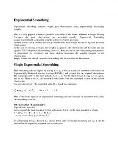
3 2 1 x 1 ? x � � � (x1 ? x) �x ? x� 77 6 ... ... ... (6) ; W ( x ) = diag K X (x) = 64 ... 5 h 1� � 1 x ? x � � � (x ? x) and e is the column vector with 1 in the tth position and zeroes elsewhere. The case p = 1 is often used in the forecasting literature for handling a local linear trend (e.g. Harvey, 1989, pp. 27{28). Figure 1 illustrates the local linear exponential smoothing forecast. p
u
e;h
p
T
u
p
T
e
T
y
t
Figure 1. Pictorial representation of Yb
time
of degree p = 1. The dotted line is tted by weighted least squares, with weights proportional to the height of the exponential function shown at the base of the plot. T
+1
The equivalent bandwidth h is a monotone transformation of the smoothing factor !. Their relationship is depicted in Figure 2 for the case x = t. One can see from this that ! = 0 corresponds to h = 0 (no smoothing) and ! = 1 corresponds to h = 1 ( tting a global pth degree polynomial). The most popular approach to automatic smoothing parameter choice in exponential smoothing is to take h, or !, to minimise the average of the squared residuals (ASR) of the previous one-step-ahead forecasts. Thus we de ne the error sum of squares choice of h, h^ ASR, as ^hASR = argmin ASR(h) �0 P where ASR(h) = T ?1 =1(Yb ? Y )2. In the next section we show that this is equivalent to choosing h by cross-validation. t
h
T t
t
t
3
1.2 1.0 0.8 omega 0.6 0.4 0.2 0.0
0
5
10
15
h
Figure 2. The relationship between ! and h. It is known that EWMA forecasting is optimal (i.e. is the minimum mean square error predictor) for the state space (or structural) model:
Y = � +" � = � ?1 + � ; t
t
t
t
t
t
where " and � are independent white noise processes. This model is sometimes referred to as a random walk plus noise. The optimality may be seen by recognising that the EWMA procedure reduces to the Kalman lter in this case (Harvey, 1989, p. 175), and it is wellknown that the Kalman lter enjoys many optimality properties for state space models. By the same token, since it is clearly not the same as the Kalman lter in other cases, EWMA is not in general an optimal procedure. This has been the source of considerable discussion in the literature about the appropriateness of using EWMA procedures when the model has not been correctly identi ed. (See Gardner, 1985, and Newbold and Bos, 1989, for example.) The optimal weights in these cases come from the Kalman lter, therefore and re ect the error structure. On the other hand a clear message from the theory of kernel smoothing is that within broad limits the choice of the kernel shape is not important, and what matters much more is getting the smoothing factor right. This reinforces the thesis of this paper that the asymptotic theory of smoothing factor selection is important. t
t
3. Asymptotic Theory We will now suppose that the data are generated according to the model
Y = m(x ) + " ; t = 1; : : : ; T t
t
t
where x = t=T and the " are realisations of a zero mean causal ARMA process (see De nitions 3.1.2 and 3.1.3 of Brockwell and Davis, 1991). Note that T ! 1 corresponds to t
t
4
the number of observations become denser in the interval [0; 1] with the dependence structure remaining the same. Let c(x) = e1 fX (x) W (x)X (x)g?1X (x) W (x)Y m � � where X (x) is the same as in (6) with x +1 replaced by x and W R(x) = diag1� � K ? for a general kernel K with the properties K (x) = 0, x > 0 and K = 1. We will refer to c(x +1). such a kernel as a half-kernel. With this notation we can rewrite (5) as Yb +1 = m While our main interest lies in forecasting Y +1, we can think of c m(x) as being a nonparametric estimate of m(x) for any x 2 [0; x +1]. But since K is a half-kernel, the estimate is always based on data to the left of x or at x itself. Our rst results concern the bias and variance of c m(x). Let N be the (p + 1) � (p + 1) matrix having (i; j ) entry equal to R u + ?2K (u) du and M (u) be the same as N , but with the rst column replaced by (1; u; : : : ; u ) . Then, as in Ruppert and Wand (1994), de ne the half-kernel K (u) = fjM (u)j=jN jgK (u): T
T
T
p
h
p
p
p
h
T
xj
h
j
T
T
x
h
T
T
T
i
p
p
j
p T
p
p
p
p
Theorem 1. Under assumptions given in the Appendix, and assuming that h = h ! 0 and Th ! 1 as T ! 1, for all x 2 [0; 1], ) ( R +1 u K ( u ) du ( +1)(x)h +1 + o(h +1 ) c(x) ? m(x)g = m E fm (p + 1)! and 9 �Z �8 1 = < X c(x)g = K (u)2 du : Varfm
(k); (Th)?1 + of(Th)?1g: T
p
p
p
p
k
p
p
=?1
c(x) has leading term Unlike ordinary local polynomial kernel smoothing, the bias of m +1 ( +1) proportional to h m (x) for both odd and even p. This is because estimation with a half-kernel corresponds to estimation at a boundary for all x (see p. 128 of Wand and Jones, 1995). For full kernels and p even this term vanishes when x is away from the boundary and a more complicated O(h +2) term becomes the leading term. A common measure of the global error in c m as an estimate of m is the Average Squared Error (ASE) X c(x ) ? m(x )g2: ASE(h) = T ?1 fm =1 c(x ) ? Y g2 in that the former is Note that ASE(h) di�ers from ASR(h) = T ?1 P =1fm c and m, while the latter is concerned with the distance concerned with the distance between m c and the time series. In nonparametric regression it is convenient to work with between m MASE(h) = E fASE(h)g: The bandwidth that minimises this quantity for a particular m is denoted by hMASE. Let 9 ( R +1 )2 Z �Z �8 1 = < X u K ( u ) du 2 2 V = K (u) du :
(k); and B = m( +1)(x)2 dx: ( p + 1)! =?1 p
p
p
T
t
t
t
T t
t
p
p
p
p
k
5
t
p
p
Then an easily derived corollary of Theorem 1 is: Corollary 1.1. Under the assumptions of Theorem 1, MASE(h) = V (Th)?1 + B 2h2 +2 + of(Th)?1 + h2 +2g p
p
p
p
and
hMASE = CMASE T ?1 (2 +3)f1 + o(1)g where CMASE = [V =f(2p + 2)B 2g]1 (2 +3). We now return to the automatic forecasting problem with smoothing factor choice based on hb ASR. For p = 0 note that, because K is a half-kernel, ?1 � x ? x � , X ?1 � x ? x � X � x ? x � , X � x ? x � X Yb = K = K h Y =1 K h h Y 6= K h =1 6= c? (x) is the same as c so hb ASR minimises P =1fY ? c m? (x )g2 where m m(x), but based on the data with (x ; Y ) omitted. The same result can be easily shown to hold for general p. Therefore, hb ASR is the same as cross-validation with a half-kernel and so its asymptotic distribution can be obtained by extending the Rresults of Chu and Marron (1991) to halfkernels and higher degree ts. Let (f � g)(x) = f (u)g(x ? u) du denote the convolution of two functions f and g. Theorem 2. Under assumptions given in the Appendix, b ASR CASR ! h 1 (4 +6) 2 T ! N (0 ; � ? ASR ): hMASE CMASE =
=
p
p
p
p
t
t
j
t
t
j
t
j
t
j
j
t
j
j
j
j
t
j
t
T t
t
t
t
t
t
t
=
p
D
where
(
P1 (k) )1 (2 +3) V ? 2 K (0) =1 CASR = ; (2p + 2)B 2 o1 (2 +3) R 2 n 4 +3 P1 Q
( k ) 8( C =C ) MASE ASR = ?1 2 = ; �ASR � � 1 (2 +3) � � 4 +5 R 2 2 2 (2p + 3) (2p + 2)B K =
p
p
p
k
p
=
p
p
p
k
=
p
p
p
Q = K � K ? ? 21 K � L? ? 12 L � K ? ? (K ? L ) p
and
p
p
p
p
K ?(u) = K (?u); p
p
p
p
p
p
L (u) = ?uK 0 (u):
p
p
p
It follows from Theorem 2 that, for large T , hb ASR ' CASRT ?1 (2 +3): In the case of independent data CASR = CMASE so hb ASR has similar asymptotic behaviour to hMASE . For the forecasting problem, there is a disturbing feature about this behaviour. It c over the entire time series. However, for means that hb ASR aims to optimise the MASE of m =
6
p
independent series the best mean squared error predictor of Y +1 is m(x +1), so the best smoothing parameter choice is one that is locally optimal for estimation of m(x +1). If instead the errors are serially correlated, for example if " = �" ?1 + u for some constant j�j < 1 and shock u independent of " ?1, then for K = K , ! CASR = 1 ? 3� 1 (2 +3) : CMASE 1+� For positive � this ratio is close to zero or even negative. This means that hb ASR is near the left end of H (de ned in the Appendix) asymptotically, which is an indication of hb ASR choosing arbitrarily small smoothing factors in the case of positive serially correlated data. Theorem 2 of Hart (1991) gives a more concise quanti cation of this behaviour. This means that hb ASR tends towards interpolation in the case of positive serial correlation. Since the most common form of exponential smoothing involves p = 0 and K = K it is also of interest to see what the asymptotic distribution of hb ASR is in this case. Corollary 2.1. For the exponentially weighted moving average forecast procedure (1), under assumptions given in the Appendix, 8 P1 (k) ? 4 P1 (k) !1 39 = < b h ASR =?1P =1 2 T 1 6 :h ? 1 ; ! N (0; �ASR)
(k) T
T
T
t
t
t
t
t
e
=
p
T
e
=
k
=
k
MASE
where
k
=?1
D
nP1 o4 3 5
( k ) = ?1 2 = o R n �ASR : 9(22 3) P1=?1 (k) ? 4 P1=1 (k) f 01 m0(x)2 dxg1 3 =
k
=
=
k
k
4. Alternative Smoothing Factor Choices Several alternatives to hb ASR which aim to remedy some of its aws are possible. For
example, the selection can be localised towards the end of the time series by inserting a weight function into the error sum of squares: �x ? x � Xb 2 (Y ? Y ) w � =1 where w is non-increasing in its negative argument and � > 0. This adaptation is a version of local cross-validation studied by and Mielniczuk, Sarda and Vieu (1989) and Hall and Schucany (1989). This modi cation addresses the localness issue, but not the dependence problem which is a much more di�cult task. The time series cross-validation method of Hart (1994) could be modi ed for this setting, but requires modelling of the covariance structure and also should be localised. Other local smoothing parameter choices with good boundary properties, such as those proposed by Fan and Gijbels (1995) and Ruppert (1997) could also be adapted to the forecast setting. A forthcoming paper by the current authors will investigate some of these possibilities. T
t
t
t
t
7
T
5. Seasonality Since seasonality is important in applications, the simple EWMA approach to forecasting described above is commonly extended to accommodate seasonal e�ects by adding recursions similar to (2) operating at a xed lag (the seasonal period). This may be done in several di�erent ways, depending on whether the seasonal e�ect is additive or multiplicative for instance, and the details may be messy, so we do not discuss these methods here. There are descriptions in the books by Harvey (1989, Section 2.2), Bowerman and O'Connell (1993, Chapter 8) and Newbold and Bos (1994, Chapter 6) for example of how this is done. (These books also contain descriptions of EWMA in practice.) Our methods and general conclusions carry over to the seasonal case. The extra features are the existence of several parameters to be determined and the possibly complex interaction between the recursions.
Acknowledgments We are grateful to Chih Kang Chu for providing us with a copy of his PhD dissertation. Research of the rst author was supported by `Projet d'Actions de Recherche Concert�ees' (No. 93/98 - 164), an FNRS-grant (No. 1.5.001.95F) and the European Human Capital and Mobility Programme (CHRX-CT94-0693) Research of the third author was supported by a grant from l'Institut de Math�ematique Pure et Appliqu�ee of Universit�e Catholiqu�e de Louvain, Belgium and by Sonderforschungsbereich 373 at Humboldt University, Germany.
Appendix Assumptions The assumptions which we make for the theorems given in this paper are:
1. m( +1) is continuous and square integrable on (0; 1). 2. K is square integrable and has compact support on the interval [?�; 0] for � > 0 such that K (0) > 0. Also, K is p + 1 times di�erentiable on its support and K ( +1) is Lipschitz continuous. 3. Data are available in the interval [?h�; 0] and are used in the construction of c m(x) This condition ensures that there are no left boundary e�ects. 4. The errors " are obtained by application of a causal linear lter (see De nition 3.1.3 of Brockwell and Davis, 1991) to independent and identically distributed random variables with mean zero and all moments nite. 5. The autocovariance function of " satis es 0 < P1=?1 (k) < 1. 6. The minimiser of P =1(Yb ?Y )2 is searched on the interval H = [aT ?1 (2 +3); bT ?1 (2 +3)] for each T , for some b > a > 0. p
p
t
t
k
T t
t
t
T
8
=
p
=
p
Proof of Theorem 1 This is a relatively straightforward extension of Theorem 4.1 of Ruppert and Wand (1994). The main di�erence is that K is now a half-kernel and so the odd order moments do not vanish. Additionally, the generalisation from independence P to causal ARMA dependence means that the variance expression has multiplicative factor 1=?1 (k) rather than the variance of the errors. See, for example, Hart (1991) for the details of such an extension. Proof of Theorem 2 Let ASR(h) = T ?1 P =1(Yb ? Y )2 denote the Average Squared Residual. The notation U = o (V ) is de ned to mean that, as T ! 1, jU =V j ! 0 almost surely and uniformly on H . Following Chu and Marron (1991) we note that k
T
t
t
T
u
t
T
T
T
T
ASR(h) = ASE(h) ? 2Cross(h) + T ?1
X T
=1
"2 + R(h) t
t
where Cross(h) = T ?1 P =1 " fYb ? m(x )g and X m(x )gfYb ? m(x ) + c m(x ) ? m(x )g: R(h) = T ?1 fYb ? c T
t
t
t
t
T
=1
t
t
t
t
t
t
t
Through straightforward calculations we have, as T ! 1, R(h) = o fMASE(h)g and 1 X Cross(h) = (Th)?1K (0) (k) + o fMASE(h)g: u
p
k
Therefore
(
ASR(h) = (Th)?1 V ? 2K (0) p
1 X
p
k
and so
=1
u
=1
)
(k) + h2 +2B 2 + o f(Th)?1 + h2 +2g p
p
u
p
hb ASR = CASRT ?1 (2 +3)f1 + o (1)g: Similarly, the minimiser of the asymptotic mean ASR, AMASR(h) = E fASE(h)?2Cross(h)+ P 2 ? 1 T =1 " g, is hAMASR = CASRT ?1 (2 +3)f1 + o(1)g: Noting that X ASR(h) = AMASR(h) + G(h) + R(h) + T ?1 f"2 ? E ("2)g =
p
u
T t
t
=
p
T
=1
t
t
t
where we have
G(h) = ASE(h) ? 2Cross(h) ? E fASE(h) ? 2Cross(h)g 0 = ASR0(hb ASR) = (hb ASR ? hAMASR )AMASR00(h�) + G0 (hb ASR) + R0(hb ASR) 9
(7)
where h� is between hb ASR and hAMASR . Using hb ASR = hAMASR f1 + o (1)g; u
and noting that AMASR00(h) = 2(Th3)?1
(
V ? 2K (0) p
1 X
p
k
we obtain
=1
)
(k) +(2p +1)(2p +2)B 2 h2 + of(Th3)?1 + h2 g p
p
p
AMASR00(h�) = C1T ?2 (2 +3)f1 + o (1)g =
p
u
where
2( 31 (2 +3) )2 1 X C1 = (2p + 3) 4 V ? 2K (0) (k) f(2p + 2)B 2g35 : =
p
p
p
k
Also,
p
p
=1
G0(hb ASR ) = G0(hAMASR ) + o fT ?(4 +3) (4 +6)g so multiplication of (7) by T (4 +3) (4 +6) gives 0 = T 3 (4 +6)(hb ASR ? hAMASR )C1 + T (4 +3) (4 +6)G0(hAMASR) + o (1): p
=
p
p
p
=
=
p
p
p
=
p
p
Theorem 2 then follows from this and, for all � > 0, 0 (X )2 Z 1 T (4 +5) (4 +6)G1(�T ?1 (2 +3)) ! N @0; (2=�)
(k) Q2 A p
=
p
=
p
D
p
k
where G1(h) = (h=2)G0 (h). This result can be obtained by re-working the arguments of Hardle, Hall and Marron (1988) for half-kernels, dependent errors and higher degree polynomial ts. A more detailed argument of this type (which treats dependent errors) can be found in Chu (1989).
References Altman, N.S. (1990) Kernel smoothing of data with correlated errors. J. Am. Statist. Assoc., 85, 749{759. Bowerman, B.L. and O'Connell, R.T. (1993). Forecasting and Time Series: an Applied Approach, Belmont: Wadsworth. Brockwell, P.J. and Davis, R.A. (1991). Time Series: Theory and Methods, Second Edition, New York: Springer. Chu, C.K. (1989). Some results in nonparametric regression. Ph.D. dissertation, Dept. Statistics, Univ. North Carolina, Chapel Hill. 10
Chu, C.K. and Marron, J.S. (1991) Comparison of two bandwidth selectors with dependent errors. Ann. Statist., 19, 1906{1918. Fan, J. and Gijbels, I. (1995) Data-driven bandwidth selection in local polynomial tting: variable bandwidth and spatial adaptation. J. R. Statist. Soc. B, 57, 371{394. Gardner, E. S. (1985) Exponential smoothing: the state of the art. J. Forecasting, 4, 1{28. Hall, P. and Schucany, W.R. (1989) A local cross-validation algorithm. Statist. Prob. Lett., 8, 109{117. Hardle, W., Hall, P. and Marron, J.S. (1988). How far are automatically chosen regression smoothing parameters from their optimum? (with discussion) J. Am. Statist. Assoc., 83, 86{101. Hart, J.D. (1991) Kernel regression estimation with time series errors. J. R. Statist. Soc. B, 53, 173{187. Hart, J.D. (1994) Automated kernel smoothing of dependent data by using time series crossvalidation. J. R. Statist. Soc. B, 56, 529{542. Harvey, A.C. (1989) Forecasting, structural time series models and the Kalman lter. New York: Cambridge University Press. Li, X. and Heckman, N.E. (1996) Local linear forecasting, unpublished manuscript. Mielniczuk, J., Sarda, P. and Vieu, P. (1989) Local data-driven bandwidth choice for density estimation. J. Statist. Plan. Inf., 23, 53{69. Newbold, P. and Bos, T. (1989) On exponential smoothing and the assumption of deterministic trend plus white noise data-generating models. Int. J. Forecasting, 5, 523{527. Newbold, P. and Bos, T. (1994) Introductory Business and Economic Forecasting, Second Edition. Cincinnati: South-Western. Ruppert, D. (1997) Empirical-bias bandwidths for local polynomial nonparametric regression and density estimation. J. Am. Statist. Assoc., to appear. Ruppert, D. and Wand, M.P. (1994) Multivariate locally weighted least squares regression. Ann. Statist., 22, 1346{1370. Wand, M.P. and Jones, M.C. (1995) Kernel Smoothing, London: Chapman and Hall.
11