Volatility Forecasting with Smooth Transition Exponential Smoothing ...

Volatility Forecasting with Smooth Transition Exponential Smoothing

James W. Taylor

International Journal of Forecasting, 2004, Vol. 20, pp. 273-286.

James W. Taylor Saïd Business School University of Oxford Park End Street Oxford OX1 1HP UK Tel: +44 (0)1865 288927 Fax: +44 (0)1865 288805 Email: [email protected]

Volatility Forecasting with Smooth Transition Exponential Smoothing

Volatility Forecasting with Smooth Transition Exponential Smoothing

Abstract Adaptive exponential smoothing methods allow smoothing parameters to change over time, in order to adapt to changes in the characteristics of the time series. This paper presents a new adaptive method for predicting the volatility in financial returns. It enables the smoothing parameter to vary as a logistic function of user-specified variables. The approach is analogous to that used to model time-varying parameters in smooth transition GARCH models. These nonlinear models allow the dynamics of the conditional variance model to be influenced by the sign and size of past shocks. These factors can also be used as transition variables in the new smooth transition exponential smoothing approach. Parameters are estimated for the method by minimising the sum of squared deviations between realised and forecast volatility. Using stock index data, the new method gave encouraging results when compared to fixed parameter exponential smoothing and a variety of GARCH models.

Key words: volatility forecasting; adaptive exponential smoothing; smooth transition; non-linear GARCH.

1. Introduction Accurate estimates of volatility are important for option pricing, portfolio analysis and risk management methodologies, such as value at risk. The observation that many financial series exhibit volatility clustering has led to the development of a great many time series methods for volatility forecasting. The two most popular time series approaches are GARCH models and smoothing methods. GARCH models enable statistical modelling of volatility. A recent development in this area has been the use of smooth transition models (see Hagerud, 1997, and GonzálezRivera, 1998). These models allow a parameter to vary over time as a continuous function of a transition variable. The sign of past shocks has been used as a transition variable in order to model the asymmetry in stock return volatility, known as the “leverage effect”. This asymmetry is characterised by the tendency for negative returns to be followed by periods of greater volatility than positive returns of equal size. The size of the past shocks has also been used as a transition variable in order to allow a more flexible modelling of the dynamics of the conditional variance. In contrast to the statistical rigour of GARCH models, smoothing methods provide a pragmatic, ad hoc approach to volatility forecasting. Exponential smoothing is a popular approach, which has been found to perform well in empirical studies (e.g. Boudoukh et al., 1997). It involves the allocation of exponentially decreasing weights to past squared shocks. Another common application of exponential smoothing is inventory control, where it is used to predict the level of a time series of demand. Researchers in this area have developed adaptive exponential smoothing methods, which allow smoothing parameters to change over time, in order to adapt to changes in the characteristics of the series (e.g. Trigg and Leach, 1967). This paper presents a new adaptive method for predicting the volatility in financial returns. It allows the smoothing parameter to vary as a logistic function of user-specified variables. The approach is analogous to that used to model the time-varying parameter in smooth transition GARCH 1

models. We propose that the same transition variables used in these models be used in the new smooth transition exponential smoothing method. We optimise the parameters in the new method by minimising the sum of squared in-sample 1-step-ahead prediction errors, where prediction error is defined as the difference between realised and forecast volatility. In our empirical work, we estimate the parameters for weekly volatility forecasting using realised weekly volatility calculated from daily data. In Section 2 we review the literature on GARCH models, including the recent work on smooth transition GARCH models. In Section 3 we introduce the new smooth transition exponential smoothing method. We describe how realised volatility can be used to estimate the parameters in the method, and we consider the method’s news impact curve. In Section 4 we use eight stock indices to compare forecasting performance of the new method to a variety of alternative methods. Section 5 provides a summary and concluding comments.

2. GARCH Models 2.1. Linear GARCH Models The most popular statistical modelling approach to volatility forecasting is Autoregressive Conditional Heteroskedasticity (ARCH) modelling, which was introduced by Engle (1982). ARCH models provide estimates of the conditional variance of the return, rt, at time t conditional upon It-1, the information set of all observed returns up to time t-1.

σ t2 = var(rt I t −1 ) This can be viewed as the variance of an error term, εt, defined by:

ε t = rt − E (rt I t −1 ) εt is often referred to as the price “shock” or “news”. ARCH models express the conditional variance as a linear function of lagged squared error terms. Bollerslev (1986) extended the ARCH class of models to Generalised Autoregressive Conditional Heteroskedastic (GARCH)

2

models, which enables a more parsimonious representation in many applications. GARCH models express the conditional variance as a linear function of lagged squared error terms and also lagged conditional variance terms. For example, the GARCH(1,1) model is given by

σ t2 = ω + α1 ε t2−1 + β1 σ t2−1

(1)

Parameters are optimised using maximum likelihood. Although the conditional distribution of returns in the likelihood function is often assumed to be Gaussian, researchers have found this to be a poor assumption and have proposed the use of the t-distribution (Bollerlev, 1987) or the generalised error distribution (Taylor, 1994). Stochastic volatility models provide an alternative volatility modelling approach (see Taylor, 1994; Shephard, 1996). However, estimation of these models has proved difficult and consequently, they are not as widely used as ARCH models.

2.2. Non-linear GARCH Models A common finding in studies of financial stock returns is that negative returns tend to be followed by periods of greater volatility than positive returns of equal size. An explanation for this asymmetry is that positive and negative shocks lead to different values for the leverage of a firm, which in turn will result in different volatilities (Black, 1976). This “leverage effect” has prompted the development of a number of GARCH models that allow for asymmetry. These models are described as non-linear because the conditional variance is no longer modelled as a linear function of lagged squared error and lagged variance. The first asymmetric formulation was the exponential GARCH model of Nelson (1991). This model uses a log formulation for volatility in order to avoid the need for non-negativity parameter constraints. The result is that the impact of lagged squared residuals is exponential, which may exaggerate the impact of large shocks. A simpler attempt to accommodate the asymmetry is the GJRGARCH model of Glosten et al. (1993). The GJRGARCH(1,1) model is given by 3

σ t2 = ω + (1 − I [ε t −1 > 0])α 1 ε t2−1 + ( I [ε t −1 > 0])γ 1ε t2−1 + β 1 σ t2−1 where I[εt-1>0] is the indicator function, taking a value of 1 if εt-1>0 and 0 otherwise. Typically, it is found that α1 > γ1, which indicates the presence of the leverage effect. A recent development in GARCH modelling has been the use of smooth transition models. The essence of these models is that at least one parameter is modelled as a continuous function of a transition variable. Franses and van Dijk (ch. 4, 2000) provide a useful review of smooth transition GARCH models. The logistic smooth transition (LSTGARCH) model of Hagerud (1997) and González-Rivera (1998) enables a smooth transition between the α and γ coefficients of the lagged squared error terms in the GJRGARCH model. The LSTGARCH(1,1) model is given by

σ t2 = ω + (1 − F (ε t −1 ))α 1 ε t2−1 + F (ε t −1 )γ 1ε t2−1 + β 1 σ t2−1 where

F (ε t −1 ) =

1 1 + exp( −θ ε t −1 )

(2)

The logistic function varies between 0 and 1, and adapts according to changes in the transition variable, εt-1. If θ > 0, the logistic function is a monotonically increasing function of εt-1. Hence, as εt-1 increases from a large negative value to a large positive value, the impact of εt-12 gradually shifts from α1 to γ1. Note that if θ is large and positive, the LSTGARCH model reduces to the GJRGARCH model. Hagerud (1997) also proposes the exponential smooth transition GARCH model (ESTGARCH). The ESTGARCH(1,1) model has the same formulation as the LSTGARCH(1,1) model, except the logistic function in expression (2) is replaced by the following exponential function: F (ε t −1 ) = 1 − exp( −θ ε t2−1 )

(3)

The exponential function enables the dynamics of the conditional variance to depend on the magnitude of the shock. This non-linear GARCH model is symmetric with respect to

4

the sign of the error term. An exponential function is used instead of a logistic because an exponential allows F(εt-1) to vary between 0 and 1 as εt-12 varies between its extremes. Rabemananjara and Zakoïan (1993) argue that conditional volatility may depend on both the sign and the size of the shock, εt-1. They suggest that the relative impacts on volatility of positive and negative shocks of equal size depend on the size, so that small positive shocks introduce more volatility than small negative ones but large negative surprises exhibit the usual leverage effect and increase volatility more than positive shocks of equal size. To accommodate this, Fornari and Mele (1997) propose a model which involves switching between two GARCH(1,1) models according to the sign of εt-1. Anderson et al. (1999) develop this idea by proposing their ANSTGARCH(1,1) model in expression (4). This model involves smooth transition between GARCH(1,1) models with F(εt-1) defined as the logistic function in expression (2).

σ t2 = (1 − F (ε t −1 ))(ω + α 1 ε t2−1 + β 1 σ t2−1 ) + F (ε t −1 )(υ + γ 1 ε t2−1 + δ 1 σ t2−1 )

(4)

3. Smooth Transition Exponential Smoothing 3.1. Exponential Smoothing A simple and popular approach to volatility forecasting is to estimate the variance as a simple moving average of past squared shocks. Boudoukh et al. (1997) write that this estimator has two clear weaknesses. Firstly, if volatility clusters, there is strong appeal to giving more recent information greater weighting, and, secondly, the choice of how many past periods to include in the moving average is arbitrary. These criticisms have led many practitioners to use an exponentially weighted moving average of as many past squared shocks as are available. With a large history of observations available, the 1-step-ahead variance estimator can be written in the simple exponential smoothing recursive form with smoothing parameter, α:

σˆ t2 = α ε t2−1 + (1 − α )σˆ t2−1

5

Exponential smoothing is also widely used to produce forecasts for the level of a time series (see Gardner, 1985). Its robustness and accuracy for short-term forecasting has led to its widespread use in applications where a large number of series necessitates an automated procedure, such as demand forecasting for inventory control. Some researchers in this area have argued that a smoothing parameter should be allowed to change over time in order to adapt to the latest characteristics of the time series. For example, if there has been a level shift in the series, the exponentially weighted average should adjust so that the weight on the most recent observations increases. A variety of adaptive exponential smoothing methods have been developed to deal with this problem (e.g. Trigg and Leach, 1967; Williams and Miller, 1999). In this paper, we introduce a new adaptive method, and apply it to volatility forecasting.

3.2. A New Adaptive Exponential Smoothing Method

We propose the use of a logistic function of a user-specified variable as adaptive smoothing parameter, and hence the method can be viewed as smooth transition exponential smoothing (STES). Applied to volatility forecasting, the method is formulated as follows:

σˆ t2 = α t −1 ε t2−1 + (1 − α t −1 )σˆ t2−1 where

α t −1 =

(5)

1 1 + exp( β + γVt −1 )

The smoothing parameter varies between 0 and 1, and adapts according to changes in the transition variable, Vt-1. As the sign and size of past shocks have been used as transition variables in non-linear GARCH models, we propose the use of εt-1 and |εt-1| as transition variables in the STES method. Although εt-12 was used as transition variable in the ESTGARCH model to represent the magnitude of the shock, there is no obvious advantage in using it in the STES method in favour of the simpler |εt-1|. An exponential function, similar to that of expression (3) for the ESTGARCH model, could be used when |εt-1| is used as 6

transition variable. However, such an exponential function would be inappropriate if εt-1 is used as transition variable because it would not restrict the smoothing parameter αt to lie between 0 and 1. For simplicity, in this paper, we use a logistic function regardless of the choice of transition variable. Clearly, if the data indicates that the smoothing parameter should be fixed, γ will be zero and the value of the fixed parameter will be set by β. Empirical results for the GARCH(1,1) model have shown that often β1≈(1-α1) in expression (1). This prompted Nelson (1990) to propose the integrated GARCH model (IGARCH), in which β1=(1-α1). This model has the appeal of robustness since fewer parameters need to be estimated. The same can be said for fixed parameter exponential smoothing, which has the same formulation as the IGARCH(1,1) model with the additional restriction that ω=0. The STES method with εt-1 as transition variable is equivalent to the ANSTGARCH(1,1) model of expression (4) with ω=0, α1=0, β1=1, υ=0, γ1=1 and δ1=0. However, this constrained formulation will not be able to capture the complex variance dynamics modelled by the unconstrained ANSTGARCH model, namely the different asymmetry for small shocks to that for large shocks. To try to overcome this, we propose the use of εt-1 and |εt-1| together as transition variables in the STES method. In Section 3.4, we plot the news impact curve for this method to gain insight into the dynamics of the method. First, we consider parameter estimation.

3.3. Parameter Estimation for Smooth Transition Exponential Smoothing As there is no statistical model underlying exponential smoothing, we are not guided by statistical theory in our choice of parameter optimisation approach. In the context of using exponential smoothing to forecast the level of a series, the forecasting literature generally recommends the minimisation of the sum of in-sample 1-step-ahead prediction errors

7

(Gardner, 1985). Since exponential smoothing for volatility forecasting is formulated in terms of variance forecasts, σˆ i2 , RiskMetrics (1996) suggests the following minimisation:

(

min ∑ ε i2 − σˆ i2

)

2

(6)

i

In this expression, the in-sample squared error, εi2, acts as a proxy for actual variance, which is unobservable. However, if interested in forecasting volatility (standard deviation), then a more suitable objective would be to minimise squared volatility prediction error. Although many authors use volatility-based cost functions to evaluate volatility forecasts (e.g. Jorion, 1995; Xu and Taylor, 1995; Boudoukh et al., 1997), the use of a volatility-based cost function to estimate parameters is rare. Perhaps the reason for this is that there is no simple proxy for actual volatility. In view of the use of εi2 as a proxy for variance, it is tempting to use |εi| as a proxy for standard deviation. However, this is unsatisfactory because |εi| will almost certainly be a biased estimator of the conditional standard deviation (Andersen and Bollerslev, 1998). In their work on evaluating variance forecasts, Andersen and Bollerslev (1998) show how higher frequency data can be used to construct realised variance, which is a better proxy for true variance than εi2. This is the approach adopted by Day and Lewis (1992) who use daily data to calculate realised weekly variance in order to evaluate variance forecasts for weekly data. Indeed, many authors calculate realised volatility from daily data in order to evaluate longer lead time forecasts (e.g. Xu and Taylor, 1995). We propose the use of higher frequency data to calculate realised volatility for use, not only in forecast evaluation, but also in parameter estimation for exponential smoothing. This proposal amounts to the parameters being derived using the following minimisation: 2 min ∑ (σ Ri − σˆ i ) i

8

(7)

where σRi is realised volatility at period i calculated from the higher frequency data. For example, if we are forecasting volatility for weekly data, realised weekly volatility could be calculated from the observations for the five trading days in the week:

σ Ri =

5

∑ε j =1

2 i −1+

j 5

(8)

A similar approach is used by Barndorff-Nielsen and Shephard (2002). They show how the parameters of stochastic volatility models for daily data can be estimated using realised volatility calculated from high frequency intra-day data. They also provide a theoretical basis for the use of realised volatility as an estimate of true volatility, which builds on the empirical studies of Andersen et al. (2000, 2001a, 2001b). Diebold (2001) reports that high frequeny data is now readily available and is being increasingly used in finance.

3.4. News Impact Curve for Smooth Transition Exponential Smoothing A useful tool for summarising and comparing volatility forecasting methods is the “news impact curve” (NIC) of Engle and Ng (1993), which has been widely used to compare different GARCH models. The curve shows the impact of shocks, or news, εt-1, on the next period’s variance forecast, σˆ t2 . In this section, we compare the NIC for the STES method using εt-1 and |εt-1| together as transition variables (STES-E&AE) with the NIC for fixed parameter exponential smoothing (ES-RVOL). We follow the approach of Anderson et al. (1999) and produce NICs corresponding to parameters estimated from real data. In the next section, we compare volatility forecasting results for a range of methods applied to eight stock indices. In this section, for simplicity, we focus solely on one of these indices, the New York S&P500 index. Although chosen arbitrarily, the features described here for this index were also evident in the NICs for the other seven indices. The sample period used to estimate the NICs consisted of 1,000 trading

9

days, from 30 December 1987 to 30 October 1991. We focused on estimating volatility in weekly log returns. The sample period delivered 200 weekly log returns. We optimised the exponential smoothing parameters using the minimisation in (7) with realised volatility calculated from daily returns as in (8). The mean of the 200 weekly returns was subtracted from each of the returns prior to estimation of the parameters. All parameter optimisations in this paper were performed using the Newton-Raphson algorithm, which is the default in Gauss, the software used in this study. The estimated parameters are shown in expression (9) below. Obviously, since there is no statistical model underlying the estimation of the parameters in exponential smoothing formulations, parameter standard errors are not produced. This is a disadvantage of the exponential smoothing methods over statistical modelling approaches, such as GARCH.

STES-E&AE

σˆ t2 = α t −1 ε t2−1 + (1 − α t −1 )σˆ t2−1 where

ES-RVOL

α t −1 =

1 1 + exp(2.07 + 7.47 ε t −1 + 14.07 ε t −1 )

(9)

σˆ t2 = 0.107 ε t2−1 + 0.893σˆ t2−1

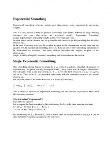
The variance forecasts are conditional on the estimate of the previous period’s variance, σˆ t2−1 . In constructing each NIC, we set σˆ t2−1 to be the unconditional variance of the 200 returns. The NICs are shown in Figure 1. The x-axis extends in both directions by three times the unconditional standard deviation of the 200 returns. ---------- Figure 1 ---------The NIC for the STES-E&AE method exhibits the complex asymmetry discussed at the end of Sections 2.2 and 3.2; small positive shocks introduce slightly more volatility than small negative shocks, but large negative shocks increase volatility more than positive shocks of equal size. Figure 1 also shows that for values of εt-1 less than zero or greater than about 0.02, the STES-E&AE NIC lies under the NIC for the ES-RVOL method, indicating that 10

STES-E&AE will often produce volatility forecasts below those from the other method. This cannot simply be due to the parameter estimation approach used because the ES-RVOL method uses the same approach. Insight can be gleaned from Figure 2, which shows the STES-E&AE smoothing parameter, given in expression (9), plotted against different values of the shock, εt-1. The plot shows that the parameter decreases as the size of the shock rises. This indicates that the dependence of the underlying conditional variance on the previous period’s squared shock is much greater for small shocks than for large. This non-linear dependence is the motivation for several of the non-linear GARCH models, such as the ESTGARCH model. The implication for the STES forecast function in expression (5) is that, as the size of the shock rises, the weight on εt-12 decreases. Figure 2 also plots the fixed parameter for the ES-RVOL method. The STES-E&AE smoothing parameter is larger than the fixed parameter only for very small shocks. In view of this, consider writing the forecast function of each of these two methods as a weighted sum of all past squared shocks. The STES-E&AE weighted sum is likely to be lower as it tends to give lower weights, than the ES-RVOL method, to all but the smallest of the squared shocks. This explains why the forecasts from the STES-E&AE method will very often be lower. ---------- Figure 2 ----------

4. Empirical Comparison of Volatility Forecasting Accuracy

4.1. Description of the Study To investigate the accuracy of the new volatility forecasting method, we carried out comparative analysis with fixed parameter exponential smoothing and a variety of GARCH models. We used stock indices from the following eight major stock markets: Amsterdam (EOE), Frankfurt (DAX), Hong Kong (Hang Seng), London (FTSE100), New York (S&P500), Paris (CAC40), Singapore (Singapore All Shares) and Tokyo (Nikkei). The sample period used in our study consisted of 2,000 trading days, from 30 December 1987 to 11

30 August 1995. We focused on forecasting volatility in weekly log returns. The sample period delivered 400 weekly log returns. For simplicity, in this initial study of smooth transition exponential smoothing, we focused solely on 1-step-ahead forecasting. We used 200 observations to estimate the parameters of the various forecasting methods. We carried out this procedure for 200 moving windows, each consisting of 200 weekly returns, to give 200 post-sample 1-step-ahead forecasts from each method. Franses and van Dijk (1996) also used four years of weekly returns to estimate parameters in their study of the accuracy of 1-step-ahead forecasts from non-linear GARCH models. We now present the 15 methods considered in our study.

4.2. Forecasting Methods GARCH Models Using Weekly Returns Although there are clearly many different GARCH models that we could have included, for reasons of practicality, we limited ourselves to the following five models, which were described earlier in the paper: GARCH, IGARCH, GJRGARCH, LSTGARCH and ESTGARCH. In a study of this nature, it is not practical to repeatedly re-specify the number of lags in the GARCH models. Therefore, we elected to use common specifications for all of the 200 moving windows. Based on the analysis of an initial data set of 200 log returns for each of the stock index series, and in view of its general popularity, we concluded that a reasonable GARCH model to use for all the series was GARCH(1,1). In view of this, we also opted for (1,1) specifications in the other GARCH models. An ARMA model can be included for the conditional mean when estimating GARCH models. Using an initial data set of 200 log returns for each of the stock index series, we found a significant AR(2) term for the Tokyo index, but no significant ARMA terms for any of the other seven series. To ensure a legitimate comparison of volatility forecasts from the different methods for the Tokyo data, we analysed volatility in the residuals from the same AR(2) model. 12

This ensured that the methods would all be applied to the same error series, εt. We derived the ARMA and GARCH parameters from the weekly returns using maximum likelihood based on a t-distribution with optimised degrees of freedom.

Fixed Parameter Exponential Smoothing Methods We implemented fixed parameter exponential smoothing using two different approaches. We optimised the parameter using the minimisation in (6) (ES-SQE) and the minimisation in (7) with realised volatility calculated from daily data as in (8) (ES-RVOL). We analysed initial series of 1000 observations for each of the daily returns on the eight indices and found autocorrelation in the Hong Kong, Singapore and Tokyo indices. In view of this, we fitted ARMA models to these three indices and used the resultant errors to calculate the realised volatility. We calculated realised volatility in the same way for these three indices throughout this study.

Smooth Transition Exponential Smoothing We implemented the STES method for three different choices of transition variables:

εt-1 (STES-E), |εt-1| (STES-AE), and εt-1 and |εt-1| together (STES-E&AE). We optimised the STES parameters using the minimisation in (7) with realised volatility defined as in (8).

GARCH Models Using Daily Returns As daily data is available, the GARCH models could be estimated using daily returns. The forecast for the volatility over a five day holding period would then serve as a forecast for weekly volatility. We implemented this approach for the following three models: GARCH(1,1), IGARCH(1,1) and GJRGARCH(1,1). We refer to these as DAILYGARCH, DAILYIGARCH and DAILYGJRGARCH. The appropriate frequency of data to use when forecasting volatility for any period is an interesting research issue. With the availability of 13

high frequency data, one could even argue that weekly volatility should not be estimated from weekly or daily returns but, instead, one should go to a much higher frequency, such as the five minute data used by Barndorff-Nielsen and Shephard (2002).

Autoregressive Models for Realised Volatility Andersen et al. (2003) show how daily exchange rate volatility can be forecasted by fitting long-memory, or fractionally-integrated, AR and VAR models to the log of realised daily volatility constructed from half-hourly returns. We included this method in our weekly volatility forecasting study, using daily returns to construct the realised weekly volatility. Following Andersen et al. (2003), we applied a long-memory filter to the log of realised weekly volatility, and then fitted an AR(5) model to the filtered data. We estimated the degree of fractional integration, d, for each moving window of 200 returns using the Geweke and Porter-Hudak (1983) log-periodogram regression estimator. We term this long-memory AR modelling of realised volatility the RV-LMAR method. The estimated values of d tended to be significantly different from zero and 0.5 for half of the eight indices, indicating long-memory stationarity. For one index, d was generally not significantly different from zero, indicating stationarity, and for the remaining three indices, d was not significantly different from 0.5, implying non-stationarity. These mixed results and the sizeable standard errors for d of about 0.08, suggest that this approach would be more suited to longer time series. Another reason for concern regarding this method was that we found far greater variability in our realised (weekly) volatility than that described by Andersen et al. (2003) in their realised (daily) volatility. This is not surprising, given that our realised (weekly) volatility was constructed from just five (daily) returns, whilst their (daily) realised volatility was calculated from 48 (half-hourly) returns. In view of this, we also fitted AR(5) models to the log realised volatility without the long-memory filter. We term this method RV-AR. 14

4.3. Post-Sample Forecasting Results Tables 1 and 2 summarise volatility forecasting performance for the 200 post-sample periods with realised weekly volatility used as proxy for actual volatility. The root mean squared error (RMSE) in Table 1 is calculated as follows: RMSE =

1 200 (σ Ri − σˆ i )2 ∑ 200 i =1

We calculated the realised weekly volatility, σRi, using the observations from the five trading days in the week, as in expression (8). The values in bold in each column of the table indicate the best performing method for each index. To summarise the relative performances of the methods across the eight series, in the final column of Table 1, we show the mean value of a Theil-U measure calculated for each series as the ratio of the RMSE for that method to the

RMSE for the STES-E&AE method. This measure has been suggested by Poon and Granger (2002). Lower values of the measure are better. Table 2 reports the coefficient of determination, R2, from the regression of realised volatility on the post-sample volatility forecasts. The regression corrects for forecast bias and so the R2 reflects the prediction error variance component of the RMSE (see Taylor, 1999a). The R2 can also be viewed as a measure of the informational content of the volatility estimator. The values in bold in each column of the table indicate the best performing method for each index. To summarise the relative performances of the methods across the eight series, in the final column of Table 2, we show the average ranking of each method. ---------- Tables 1 and 2 ---------Overall, the IGARCH and GJRGARCH models were the best performing of the five GARCH models estimated using weekly returns. The IGARCH performance indicates that there is value in imposing the constraint β1=(1-α1) on the GARCH(1,1) formulation in expression (1). The GJRGARCH results confirm the belief that there is a sizeable leverage effect in stock returns. The results for the LSTGARCH and ESTGARCH model are disappointing, suggesting 15

that they are no better than the linear GARCH model for 1-step-ahead forecasting. The GARCH models, estimated using weekly data, did not outperform exponential smoothing with fixed parameter estimated from the same data (ES-SQE). Statistically sophisticated methods have also failed to outperform exponential smoothing in various competitions comparing the accuracy of forecasts for the level of a series (e.g. Makridakis and Hibon, 2000). Interestingly, the GJRGARCH(1,1) model estimated using daily returns (DAILYGJRGARCH) outperforms all five GARCH models estimated using weekly returns. The extra information supplied by the higher frequency data is clearly beneficial for the GJRGARCH model. The results were mixed for the autoregressive modelling of realised volatility, inspired by Andersen et al. (2003). The long-memory RV-LMAR method performed poorly, particularly in respect of the R2 measure. As we discussed in Section 4.2, this method is probably more suited to longer series and higher frequency data. By contrast, the simpler AR modelling of log realised volatility, the RV-AR method, performed very well in terms of RMSE and quite competitively in terms of the R2 measure. The results in Tables 1 and 2 for the STES-E method are similar to those for the two fixed parameter exponential smoothing methods. The case for the other two smooth transition exponential smoothing methods is more convincing. Using εt-1 and |εt-1| together as transition variables (STES-E&AE) was more successful than using just |εt-1| (STES-AE). The STESE&AE method has the best R2 mean rank in Table 2, and has jointly the best mean Theil-U measure for the RMSE results in Table 1. It is important to note that the high performance of the STES-E&AE method cannot simply be the result of the parameter estimation approach because the method comfortably outperforms the ES-RVOL method, which uses the same approach. It could be argued that, by using realised volatility calculated from daily returns in the evaluation measures, the GARCH methods, estimated using weekly returns, are at a disadvantage. For completeness, in Tables 3 and 4, we show how the methods perform when

16

variance is evaluated using εi2 as a proxy for actual variance in week i. RMSE in Table 3 was calculated as follows:

RMSE =

1 200

∑ (ε 200 i =1

2 i

− σˆ i2

)

2

---------- Tables 3 and 4 ---------While there is little to choose between the methods in Table 3, the relative performances of the methods in Table 4 are broadly similar to those in Tables 1 and 2. One point to note is that, in Tables 3 and 4, as one might have expected, the performances of the GARCH models estimated using weekly returns, relative to the same models estimated using daily observations, has improved from that in Tables 1 and 2. We also evaluated the variance forecasts using realised variance, calculated from daily returns, as a proxy for actual variance in the calculation of the evaluation measures. We do not report the results here because the relative performances of the methods were similar to that shown in Tables 1 to 2 for realised standard deviation. We have used |εt-1| as transition variable in the STES method because it is the simplest representation of the magnitude of the previous period’s shock. However, we should point out that using εt-12, instead of |εt-1|, led to similar volatility forecasting accuracy.

5. Summary and Conclusion

Exponential smoothing is a popular, pragmatic approach to volatility forecasting. In this paper, we have introduced a new smooth transition exponential smoothing method that uses a logistic function as adaptive smoothing parameter. We propose the use of εt-1 and |εt-1| as transition variables in order to try to replicate the conditional variance dynamics of the smooth transition GARCH models. We propose that parameters for the method be estimated by minimising the sum of squared deviations between realised and forecast volatility. In our work, we estimated the parameters for weekly volatility forecasting using realised weekly volatility calculated from daily data. With the increasing availability of high frequency data, 17

intra-day data can be used to calculate realised daily volatility for use in the estimation of parameters for daily volatility forecasting. Using eight stock indices, we compared the accuracy of weekly volatility forecasts from the new approach to fixed parameter exponential smoothing, a range of GARCH models and autoregressive models for realised volatility. The results were very encouraging for the new smooth transition exponential smoothing method with εt-1 and |εt-1| together as transition variables. The news impact curve for this method shows the complex asymmetric behaviour initially suggested by Rabemananjara and Zakoïan (1993); small positive shocks introduce more volatility than small negative ones, but large negative surprises exhibit the usual leverage effect by increasing volatility more than positive shocks of equal size. Another method that performed very well in the empirical comparison was an AR model for log realised volatility, which was inspired by the recent work of Andersen et al. (2003). In this introductory paper, we have focused solely on 1-step-ahead forecasting. An interesting issue for further research is multi-step-ahead forecasting from the new STES method. Franses and van Dijk (p. 194, 2000) note that for some non-linear GARCH models, such as ESTGARCH, analytic expressions for the multi-step-ahead conditional variance forecast do not exist, in which case simulation must be used to generate the forecasts. Analytic expressions also do not exist for smooth transition exponential smoothing when |εt-1| or εt-12 are used as transition variables. With fixed parameter exponential smoothing, a popular approach to forecasting volatility over a k-period holding period is to multiply the 1step-ahead forecast by k½. However, a number of authors have warned against this (e.g. Diebold et al., 1998), showing that it can often substantially misestimate the volatility. An alternative is to adapt the nonparametric methods of Taylor (1999b, 2000) to find a more appropriate inflationary factor than k½.

18

Acknowledgements

We would like to thank Philip Hans Franses and Dick van Dijk for making the data available. We are also grateful for the useful comments of three anonymous referees.

References

Andersen, T.G., & Bollerslev, T. (1998). Answering the Critics: Yes, ARCH models do provide good volatility forecasts, International Economic Review, 39, 885-906. Andersen, T.G., Bollerslev, T., Diebold, F.X., & Ebens, H. (2001a). The distribution of realized stock return volatility, Journal of Financial Economics, 61, 43-76. Andersen, T.G., Bollerslev, T., Diebold, F.X., & Labys, P. (2000). Exchange rate returns standardised by realised volatility are (nearly) Gaussian, Multinational Finance Journal, 4, 159-179. Andersen, T.G., Bollerslev, T., Diebold, F.X., & Labys, P. (2001b). The distribution of realized exchange rate volatility, Journal of the American Statistical Association, 96, 42-55. Andersen, T.G., Bollerslev, T., Diebold, F.X., & Labys, P. (2003). Modeling and Forecasting Realized Volatility, forthcoming, Econometrica. Anderson, H.M., Nam, K., & Vahid, F. (1999). Asymmetric nonlinear smooth transition GARCH models. In: P. Rothman (Ed.), Nonlinear Time Series Analysis of Economic and Financial Data (pp. 191-207). Boston: Kluwer. Barndorff-Nielsen, O.E., & Shephard, N. (2002). Econometric analysis of realised volatility and its use in estimating stochastic volatility models. Journal of the Royal Statistical Society, Series B, 64, 253-280. Black, F. (1976). The pricing of commodity contracts, Journal of Financial Economics, 3, 167-179. Bollerslev, T. (1986). Generalized autoregressive conditional heteroskedasticity, Journal of Econometrics, 31, 307-327. Bollerslev, T. (1987). A conditionally heteroskedastic time series model for speculative prices and rates of return, Review of Economics and Statistics, 69, 542-547. Boudoukh, J., Richardson, M., & Whitelaw, R.F. (1997). Investigation of a class of volatility estimators, Journal of Derivatives, 4 Spring, 63-71. Day, T.E., & Lewis, C.M. (1992). Stock market volatility and the informational content of stock index options, Journal of Econometrics, 52, 267-287. Diebold, F.X. (2001). Econometrics: Retrospect and prospect, Journal of Econometrics, 100, 73-75. 19

Diebold, F.X., Hickman, A., Inoue, A., & Schuermann, T. (1998). Scale models. Risk, January, 104-107. Engle, R.F. (1982). Autoregressive conditional heteroscedasticity with estimates of the variance of United Kingdom inflation, Econometrica, 50, 987-1008. Engle, R.F., & Ng, V.K. (1993). Measuring and testing the impact of news on volatility, Journal of Finance, 48, 1749-1778. Fornari, F., & Mele, A. (1997). Sign- and volatility switching ARCH models: theory and applications to international stock markets, Journal of Applied Econometrics, 12, 49-65. Franses, P. H., & van Dijk, D. (1996). Forecasting stock market volatility using (non-linear) GARCH models, Journal of Forecasting, 15, 229-235. Franses, P. H., & van Dijk, D. (2000). Non-Linear Time Series Models in Empirical Finance. Cambridge, UK: Cambridge University Press. Gardner, E.S., Jr. (1985). Exponential smoothing: the state of the art, Journal of Forecasting, 4, 1-28. Geweke, J., & Porter-Hudak, S. (1983). The Estimation and Application of Long Memory Time Series Models, Journal of Time Series Analysis, 4, 221-238. Glosten, L.R., Jagannathan, R., & Runkle, D.E. (1993). On the relation between the expected value and the volatility of the nominal excess return on stocks, Journal of Finance, 48, 17791801. González-Rivera, G. (1998). Smooth transition GARCH models, Studies in Nonlinear Dynamics and Econometrics, 3, 61-78. Hagerud, G.E. (1997). A New Non-Linear GARCH Model. PhD thesis, IFE, Stockholm School of Economics. Jorion, P. (1995). Predicting volatility in the foreign exchange market, Journal of Finance, 50, 507-528. Makridakis, S., & Hibon, M. (2000). The M3-Competition: results, conclusions and implications, International Journal of Forecasting, 16, 451-476. Nelson, D.B. (1990). Stationarity and persistence in the GARCH(1,1) model, Econometric Theory, 6, 318-334. Nelson, D.B. (1991). Conditional heteroskedasticity in asset returns: a new approach, Econometrica, 59, 347-370. Poon, S., & Granger, C.J.W. (2003). Forecasting Volatility in Financial Markets: A Review, Journal of Economic Literature, forthcoming, 2003. Rabemananjara, R., & Zakoïan, J.M. (1993). Threshold ARCH models and asymmetries in volatility, Journal of Applied Econometrics, 8, 31-49. 20

RiskMetrics (1996). RiskMetricsTM Technical Document. Fourth edition, J.P. Morgan/Reuters. Shephard, N.G. (1996). Statistical aspects of ARCH and stochastic volatility. In: D.R. Cox et al. (Eds.), Time Series Models: In Econometrics, Finance and Other Fields (Chapter 1, pp. 1-67). New York: Chapman & Hall. Taylor, J.W. (1999a). Evaluating volatility and interval forecasts, Journal of Forecasting, 18, 111-128. Taylor, J.W. (1999b). A quantile regression approach to estimating the distribution of multiperiod returns, Journal of Derivatives, 7 Fall, 64-78. Taylor, J.W. (2000). A quantile regression neural network approach to estimating the conditional density of multiperiod returns, Journal of Forecasting, 19, 299-311. Taylor, S.J. (1994). Modelling stochastic volatility: a review and comparative study, Mathematical Finance, 4, 183-204. Trigg, D.W., & Leach, A.G. (1967). Exponential smoothing with an adaptive response rate, Operational Research Quarterly, 18, 53-59. Williams, D.W., & Miller, D. (1999). Level-adjusted exponential smoothing for modeling planned discontinuities, International Journal of Forecasting, 15, 273-289. Xu, X., & Taylor, S.J. (1995). Conditional volatility and the informational efficiency of the PHLX currency options market, Journal of Banking and Finance, 19, 803-821.

21

σˆ t2

0.00065

0.00055

0.00045

-0.06

-0.04

-0.02

0.00035 0.00

STES-E&AE

ε t-1 0.02

0.04

ES-RVOL

Figure 1: News impact curves for smooth transition exponential smoothing (STES-E&AE) and fixed parameter exponential smoothing (ES-RVOL) applied to 200 weekly log returns of the S&P 500 index.

22

0.06

α t-1 0.12 0.10

0.08

0.06

0.04

0.02

-0.06

-0.04

-0.02

0.00 0.00

STES-E&AE

ε t-1 0.02

0.04

0.06

ES-RVOL

Figure 2: Smoothing parameter for smooth transition exponential smoothing (STES-E&AE) and fixed parameter exponential smoothing (ES-RVOL) applied to 200 weekly log returns of the New York S&P 500 index.

23

Amsterdam Frankfurt Hong Kong London New York

Paris

Singapore Tokyo Mean Theil

GARCH

0.77

0.86

1.52

0.89

0.66

0.90

1.09

1.44

1.14

IGARCH

0.72

0.88

1.52

0.85

0.66

0.88

1.05

1.34

1.10

GJRGARCH

0.73

0.88

1.52

0.85

0.66

0.88

1.05

1.35

1.11

LSTGARCH

0.75

0.87

1.54

0.87

0.66

0.90

1.07

1.48

1.13

ESTGARCH

0.87

0.93

1.75

0.88

0.67

0.97

1.21

1.45

1.22

DAILYGARCH

0.69

0.78

1.56

0.74

0.61

0.88

1.03

1.39

1.06

DAILYIGARCH

0.73

0.81

1.77

0.76

0.60

0.97

1.04

1.39

1.10

DAILYGJRGARCH

0.69

0.78

1.53

0.73

0.58

0.87

0.98

1.31

1.03

RV-LMAR

0.68

0.86

1.75

0.75

0.59

0.92

0.93

1.57

1.09

RV-AR

0.64

0.72

1.61

0.71

0.57

0.88

0.86

1.32

1.00

ES-SQE

0.72

0.81

1.65

0.85

0.63

0.90

0.98

1.43

1.10

ES-RVOL

0.75

0.82

1.54

0.86

0.62

0.94

0.96

1.44

1.10

STES-E

0.76

0.82

1.53

0.80

0.62

0.94

0.97

1.38

1.09

STES-AE

0.67

0.76

1.54

0.75

0.58

0.91

0.90

1.40

1.03

STES-EAE

0.65

0.76

1.45

0.73

0.57

0.91

0.85

1.35

1.00

Table 1: RMSE for 200 post-sample weekly volatility forecasts using realised volatility as actual.

Amsterdam Frankfurt Hong Kong London New York

Paris

Singapore Tokyo Mean rank

GARCH

9.4

10.6

22.1

2.8

5.2

3.3

7.5

24.9

9.0

IGARCH

12.7

10.4

20.1

0.9

4.6

7.1

7.6

30.7

7.8

GJRGARCH

12.1

11.0

20.4

1.1

4.9

7.2

7.8

29.2

7.4

LSTGARCH

8.6

8.5

20.0

0.4

5.4

2.9

6.6

24.2

11.5

ESTGARCH

8.7

10.8

9.7

0.6

6.7

3.2

8.0

27.2

9.4

DAILYGARCH

6.9

14.7

14.5

9.8

6.1

4.4

12.4

28.2

7.1

DAILYIGARCH

8.3

15.7

15.6

8.4

6.6

3.8

17.4

28.6

5.3

DAILYGJRGARCH

6.5

14.8

17.0

11.6

6.7

5.7

15.4

29.3

5.3

RV-LMAR

2.7

9.6

5.5

1.7

3.9

0.5

0.1

1.9

14.1

RV-AR

6.8

17.1

15.2

12.8

4.4

3.4

11.7

30.1

7.3

ES-SQE

7.3

11.0

11.3

0.7

6.0

3.4

8.5

23.4

10.1

ES-RVOL

7.8

13.9

26.1

0.0

6.0

3.1

13.0

29.3

7.6

STES-E

7.0

13.7

20.8

6.4

5.9

2.8

11.9

33.0

7.3

STES-AE

9.6

14.4

17.6

4.6

6.5

2.1

8.2

31.7

6.9

STES-EAE

11.1

14.8

24.7

8.2

6.3

3.2

14.6

33.0

4.1

Table 2: R2 for 200 post-sample weekly volatility forecasts using realised volatility as actual. R2 values are percentages.

24

Amsterdam Frankfurt Hong Kong London New York 2255

889

398

Paris 793

Singapore Tokyo Mean Theil

GARCH

530

735

624

2107

IGARCH

533

737

2231

884

404

784

625

2023

1.00

GJRGARCH

531

735

2233

887

403

784

623

2025

1.00

LSTGARCH

527

742

2266

885

399

793

626

2141

1.01

ESTGARCH

552

746

2307

882

398

811

655

2118

1.02

DAILYGARCH

529

725

2323

878

387

791

671

2089

1.01

DAILYIGARCH

536

733

2507

885

386

817

749

2097

1.04

DAILYGJRGARCH

530

724

2321

877

385

783

653

2073

1.00

RV-LMAR5

536

748

2362

895

389

825

637

2180

1.02

RV-AR5

535

730

2318

890

390

808

627

2083

1.01

ES-SQE

521

731

2280

882

391

800

620

2105

1.00

ES-RVOL

529

738

2332

887

394

809

625

2153

1.01

STES-E

531

739

2269

887

394

811

622

2119

1.01

STES-AE

525

738

2277

892

390

813

628

2135

1.01

STES-EAE

527

735

2255

889

388

809

623

2091

1.00

1.00

Table 3: RMSE for 200 post-sample weekly variance forecasts using εi2 as actual. RMSE values have been multiplied by 106.

Amsterdam Frankfurt Hong Kong London New York

Paris

Singapore Tokyo Mean rank

GARCH

0.6

0.1

1.9

1.5

1.3

0.1

1.7

7.1

8.5

IGARCH

0.3

1.2

3.0

0.1

0.7

1.8

1.3

11.9

7.4

GJRGARCH

0.4

1.4

2.9

0.3

0.7

1.7

1.5

11.8

6.3

LSTGARCH

0.5

0.0

1.5

0.6

1.2

0.1

0.9

6.4

11.8

ESTGARCH

0.5

0.2

0.3

1.3

2.2

0.1

2.1

6.9

9.1

DAILYGARCH

0.0

0.8

0.6

0.9

3.0

1.2

0.7

7.0

8.9

DAILYIGARCH

0.2

0.9

0.5

0.3

3.2

1.2

1.4

6.7

8.8

DAILYGJRGARCH

0.0

1.0

0.8

1.3

3.7

2.3

1.1

7.9

7.3

RV-LMAR5

0.2

1.3

1.5

0.1

1.6

0.9

0.0

1.3

10.1

RV-AR5

0.2

1.9

2.3

0.8

1.5

0.7

3.3

9.3

5.6

ES-SQE

1.0

0.3

0.9

1.6

2.3

0.1

1.3

6.5

8.1

ES-RVOL

0.8

0.3

2.2

1.8

1.6

0.3

2.9

6.8

6.5

STES-E

0.7

0.2

2.0

0.0

1.5

0.2

3.0

8.3

8.4

STES-AE

1.1

0.2

2.3

0.1

2.2

0.1

1.3

8.1

8.4

STES-EAE

1.1

0.7

3.2

0.3

2.3

0.4

2.8

8.7

5.0

Table 4: R2 for 200 post-sample weekly variance forecasts using εi2 as actual. R2 values are percentages.

25