1. INTRODUCTION. Joint factor analysis (JFA) [1, 2, 3] has contributed to state-of-the-art ..... Also as shown in Table 4 (ID 6 vs 5), after fusing with. JFA baseline ...
SPEAKER VERIFICATION USING SIMPLIFIED AND SUPERVISED I-VECTOR MODELING Ming Li, Andreas Tsiartas, Maarten Van Segbroeck and Shrikanth S. Narayanan Signal Analysis and Interpretation Laboratory, University of Southern California, Los Angeles, USA ABSTRACT This paper presents a simplified and supervised i-vector modeling framework that is applied in the task of robust and efficient speaker verification (SRE). First, by concatenating the mean supervector and the i-vector factor loading matrix with respectively the label vector and the linear classifier matrix, the traditional i-vectors are then extended to label-regularized supervised i-vectors. These supervised ivectors are optimized to not only reconstruct the mean supervectors well but also minimize the mean squared error between the original and the reconstructed label vectors, such that they become more discriminative. Second, factor analysis (FA) can be performed on the pre-normalized centered GMM first order statistics supervector to ensure that the Gaussian statistics sub-vector of each Gaussian component is treated equally in the FA, which reduces the computational cost significantly. Experimental results are reported on the female part of the NIST SRE 2010 task with common condition 5. The proposed supervised i-vector approach outperforms the i-vector baseline by relatively 12% and 7% in terms of equal error rate (EER) and norm old minDCF values, respectively. Index Terms— Speaker verification, Simplified i-vector, Supervised i-vector 1. INTRODUCTION Joint factor analysis (JFA) [1, 2, 3] has contributed to state-of-the-art performance in text independent speaker verification (SRE). It is a powerful and widely used technique for compensating the variability caused by different channels and sessions. Recently, total variability i-vector modeling has gained significant attention in SRE due to its excellent performance, low complexity and small model size [4]. In this approach, a single factor analysis is firstly used as a front-end to generate a low dimensional total variability space (i.e. the i-vector space) which jointly models speaker and channel variabilities [4]. Within the i-vector space, variability compensation methods, such as Within-Class Covariance Normalization (WCCN) [5], Linear Discriminative Analysis (LDA) and Nuisance Attribute Projection (NAP) [6], are performed to reduce the variability for the subsequent probabilistic LDA (PLDA) modeling [7, 8]. Since i-vectors cover speaker and channel variabilities all together as one unsupervised method, these variability compensation methods are required in the back end. This motivates us to investigate a joint optimization to minimize the weighted sum of both the re-construction and the classification error simultaneously. In this work, the traditional i-vectors are extended to the label regularized supervised i-vectors by concatenating the mean supervector and the i-vector factor loading matrix, respectively with the label vector and the linear classifier matrix at the end. Compared to the traditional i-vectors, this joint optimization can discriminatively select the top eigen directions related to the given labels such that the This work was supported in part by NSF and DARPA.
978-1-4799-0356-6/13/$31.00 ©2013 IEEE
non-relevant information is reduced in the i-vector space (e.g. noise, variabilities from undesired sources) and performance is improved. Moreover, the i-vector training and extraction algorithms are computationally expensive which limits practical usage, especially for large sized GMM model and data set [9, 10]. Both [10] and [9] used pre-calculated Universal Background Model (UBM) weighting vector to approximate each utterance’s 0th order GMM statistics vector to avoid the computationally expensive GMM componentwise matrix operations in the SRE task. This approximation resulted a processing speed up by a factor 10 to 25 at the cost of a significant performance degradation (17% EER) [9]. By enforcing the approximation at both training and extraction stage, the performance degradation can be reduced [10] in condition where no or very little mismatch between train/test data and UBM data exists. In this work, we investigated an alternative robust and efficient solution which is not based on the UBM weights vector. We performed factor analysis (FA) on the pre-normalized GMM first order statistics supervector to ensure each Gaussian component’s statistics sub-vector is treated equally in the FA which reduces the computational cost by a factor 40. This way, each utterance is represented by a single pre-normalized supervector as the feature vector plus one total frame number to control its importance against the prior. Each component’s statistics sub-vector is normalized by its own occupancy probability square root, thus it avoids the mismatch between global pre-calculated average weighting vector ([10] adopted the UBM weights) and each utterance’s own occupancy probability distribution vector. Furthermore, since there is only a global total frame number inside the matrix inversion, we can create a global cache table of the resulting matrices against its log value. The log domain is chosen since the smaller the total frame number, the more important it is against the prior. By looking at the table, the speed of extracting an i-vector for each sentence can be increased by another 3 times at the cost of a small quantization error. The larger the table, the smaller this quantization error. 1.1. Relation to prior work First, the traditional i-vector approach [4] is extended to the labelregularized supervised i-vector framework to improve the performance. Second, an alternative simplified approximation method is provided for both i-vector and supervised i-vector modeling. The difference with [9, 10] is that our method does not rely on the UBM weights vector. Third, although this simplified supervised i-vector method was also introduced in another submission (language identification on highly noisy data [11]), its application on the SRE task and traditional NIST environment is new. As an extension to the work of [11], we demonstrate that the design of both the label vector and classification matrix can be flexibly changed regarding different applications (such as identification versus verification). We propose another new design with speaker specific sample mean i-vector as the label vector especially for verification purpose in this work.
7199
ICASSP 2013
2. METHODS 2.1. The i-vector (IV) baseline In the total variability space, there is no distinction between the speaker effects and the channel effects. Rather than separately using the eigenvoice matrix V and the eigenchannel matrix U [1], the total variability space simultaneously captures the speaker and channel variabilities [4]. Given a C component GMM UBM model λ with λc = {pc , µc , Σc }, c = 1, · · · , C and an utterance with a L frame feature sequence {y1 , y2 , · · · , yL }, the 0th and centered 1st order Baum-Welch statistics on the UBM are calculated as follows: Nc =
L X
P (c|yt , λ)
(1)
P (c|yt , λ)(yt − µc )
(2)
t=1
Fc =
L X t=1
where c = 1, · · · , C is the GMM component index and P (c|yt , λ) is the occupancy probability for yt on λc . The corresponding cen˜ is generated by concatenating all the F˜c tered mean supervector F together: PL t=1 P (c|yt , λ)(yt − µc ) ˜ . (3) Fc = PL t=1 P (c|yt , λ) ˜ can be projected as follows: The centered GMM mean supervector F ˜ = Tx, F
classifier matrix at the end of the mean supervector and the i-vector factor loading matrix, respectively. These supervised i-vectors are optimized not only to reconstruct the mean supervectors well but also to minimize the mean square error between the original and the reconstructed label vectors, and thus can make the supervised ivectors become more discriminative in terms of the regularized label information. F˜j Lj
» P (xj ) = N (0, I), P (
–
» |xj ) = N (
In (6,7,8), xj , Nj , F˜j and Lj denote the j th utterance’s i-vector, N matrix, mean supervector and label vector, respectively. Σ1 and Σ2 denote the variance for CD dimensional mean P supervector and M dimensional label vector, respectively. nj = C c=1 Ncj where Ncj denotes the Nc for the j th utterance. The reason for using a global scalar nj is that each label vector dimension is treated equally in terms of frame length importance, the variance Σ2 is adopted to capture the variance of label vectors. We define two types of label vectors as follows: 1 if utterance j is from class i Supervised type 1: Lij = 0 otherwise (9) For type 1 label vectors, we want the regression matrix W to correctly classify the class labels. Suppose there are M speaker classes, Lj is a M dimensional binary vector with only one non-zero element with the value of 1 and W is a M × K linear classification matrix. Lj = x ¯sj , W = I.
Supervised type 2:
˜ x = (I + Tt Σ−1 NT)−1 Tt Σ−1 NF
Γ X
ln(P (F˜j , Lj , xj )) =
j=1
P (F˜j |xj ) = N (Txj , N−1 j Σ)
(6)
therefore, the posterior distribution of i-vector x given the observed ˜ for the j th utterance is: F Nj T)
−1
t
T Σ
−1
t
˜j , (I + T Σ Nj F
j=1
(12)
− 12 ln(|Σ1 −1 |) + 12 (Lj − Wxj )t Σ2 −1 nj (Lj − Wxj ) − 21 ln(|Σ2 −1 |))
The i-vector training and extraction can be re-interpreted as a classic factor analysis based generative modeling problem. For the j th utterance, the prior and the conditional distribution is defined as following multivariate Gaussian distributions:
−1
– » Γ X F˜j |xj )) + ln(P (xj ))} {ln(P ( Lj
(11) Combining (10) and (11) together and removing non-relevant items, we can get the objective function J for the Maximum Likelihood (ML) EM training: P t −1 1 t 1 ˜ J= Γ Nj (F˜j − Txj ) j=1 ( 2 xj xj + 2 (Fj − Txj ) Σ1
2.2. Label-regularized supervised i-vector (SUP-IV)
t
(10)
Type 2 label vectors are the sample mean vector of all the supervised i-vectors from the same speaker index in the last iteration x ¯sj (similar to the one in WCCN). The reason is to reduce the within class covariance and help all the supervised i-vectors to move towards their class sample mean. Therefore, M = K in this case. The log likelihood of the total Γ utterances is:
(5)
where N is a diagonal matrix of dimension CD × CD whose diagonal blocks are Nc I, c = 1, · · · , C and Σ is a diagonal covariance matrix of dimension CD×CD estimated in the factor analysis training step. It models the residual variability not captured by the total variability matrix T [4]. Covariance Σ is also updated iteratively.
˜j ) = N ((I + T Σ P (xj |F
# – " N−1 j Σ1 ) , n−1 j Σ2 (8)
(4)
where T is a rectangular total variability matrix of low rank and x is the so-called i-vector [4]. Considering a C-component GMM and D dimensional acoustic features, the total variability matrix T is a CD × K matrix which can be estimated the same way as learning the eigenvoice matrix V in [12] except that here we consider that every utterance is produced by a new speaker [4]. ˜ and total variability maGiven the centered mean supervector F trix T, the i-vector is computed as follows [4]:
P (xj ) = N (0, I),
Txj Wxj
−1
Nj T)
The solution is as follows: E(xj )
(I + Tt Σ1 −1 Nj T + Wt Σ2 −1 nj W)−1 (Tt Σ1 −1 Nj F˜j + Wt Σ2 −1 nj Lj ), (13)
=
E(xj xj t ) = E(xj )E(xj )t + (I + Tt Σ1 −1 Nj T + Wt Σ2 −1 nj W)−1 . (14) Γ Γ X X t t −1 Type 1: Wnew = [ nj Lj E(xj )][ nj E(xj xj )] (15) j=1
−1
). (7)
The mean of the posterior distribution (point estimate) is adopted as the i-vector which is the same as equation (5). The traditional i-vectors are extended to the label-regularized supervised i-vectors by concatenating the label vector and the linear
j=1
For the T matrix, we employed the strategy used in [4] to update component by component since Ncj is also a scalar.
7200
Tcnew = [
Γ X
j=1
Ncj F˜cj E(xj t )][
Γ X j=1
Ncj E(xj xj t )]−1
(16)
In (16), Tc denotes the [(c − 1)D + 1 : cD] rows sub-matrix of T and F˜cj is the [(c − 1)D + 1 : cD] elements sub-vector of F˜j .
Type 1: Type 2:
Σ2 = Σ2 =
˜ − Tnew E(xj ))F˜j t )}
PΓ
j=1 (Nj (Fj
Γ diag{ diag{
PΓ
j=1 (nj (Lj
− Wnew E(xj ))Lj t )}
(17) (18)
Γ (n (L − E(xj ))t (Lj − E(xj )))} j j j=1
PΓ
Γ
(19)
These 2 variance vectors describe the energy that can not be represented by factor analysis and control the importance in the joint optimization objective function (12). Σ2 for the type 2 label vectors is just the diagonal elements of the within class covariance matrix in WCCN. After several iterations of EM training, the parameters are learned. For the subsequent supervised i-vector extraction, we let Σ2 to be infinity since we do not know the ground truth label information. This will revert equation (13) back to equation (5). After the supervised i-vector extraction, the classification methods steps are the same as in the traditional i-vector modeling. There are some obvious extensions of this supervised i-vector framework. We can make L as the parameter vector that we want to perform regression with (e.g. ages [13, 14], paralinguistic measures [15]) to make the proposed framework suitable for regression problems. Moreover, if the classification or regression relation is not linear, we can use non-linear mapping as a preprocessing step before generating L.
I-vector training and extraction is computationally expensive. Let the GMM size, feature dimension, factor loading matrix size to be C, D, and K, respectively. The complexity for generating a single i-vector is O(K 3 + K 2 C + KCD) [10]. In this work, we make two approximations to reduce the complexity. The K 3 term comes from the matrix inversion while the K 2 C term is from Tt Σ−1 Nj T in equation (5). When C is large, this K 2 C term’s computational cost is huge. The fundamental reason is that each Gaussian component λc has different Nc for each utterance j which means some sub-vectors F˜cj have less variance than others in F˜j and need utterance specific intra mean supervector reweighting in the objective function. We first decompose the Nj vecP tor into Nj = nj mj where nj = C c=1 Ncj , mcj = Ncj /nj and PC m = 1. m is the re-weighting vector and nj (total frame cj j c=1 number) controls the confidence at the global level. Our motivation is to re-weight each utterance’s mean supervector with its own (mj )1/2 before the factor analysis step which makes each dimension of the new supervector Fˆj be treated equally in the approximated modeling (21,22). PL
P (c|yt , λ)(yt − µc ) Ncj 1 ˆ [ ] 2 , Fj = mj 1/2 F˜j PL nj t=1 P (c|yt , λ)
t=1
(20)
So the intra supervector imbalance is compensated by this preweighting, and each utterance is represented by Fˆj as the general feature vector and nj as the confidence value for the subsequent machine learning algorithms. We perform factor analysis in the following way by linearly projecting this new normalized supervector ˆ on a dictionary T: ˆ F ˆ = Tx, ˆ P (xˆj ) = N (0, I) F ˆ xˆj , mj (nj mj )−1 Σ) = N (T ˆ xˆj , n−1 Σ) P (Fˆj |xˆj ) = N (T j
4
3
2
1
0 0
50
100
150
200
250
300
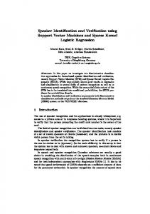
Table Index Fig. 1. The nj quantization curve in the log domain, 300 indexes. Table 1. Complexity of the proposed methods for a single utterance (GMM size C = 1024, feature dimension D = 36, T matrix rank K = 500, table index size is 300, label vector dimension M = 2543, 500 (type 1,2), time was measured on a Intel I7 CPU with a single thread and 12 GB memory ) Methods Approximated complexity Time IV O(K 3 + K 2 C + KCD) 2.82s Type 1 SUP-IV O(K 3 + K 2 C + K(CD + M )) 2.85s SIM-IV without table O(K 3 + KCD) 0.062s SIM-IV with table O(KCD) 0.022s SIM-SUP-IV without table O(K 3 + K(CD + M )) 0.066s SIM-SUP-IV with table O(K(CD + M )) 0.023s
ˆ given the obTherefore, the posterior distribution of the i-vector x ˆ is: served F
2.3. Simplified i-vector (SIM-IV)
Fˆc =
x 10
j
diag{
Corresponding n value
Σ1 =
4
(21) (22)
−1 ˆ −1 Tˆt Σ−1 nj Fˆj ), (I + Tˆt Σ−1 nj T) ˆ −1 ). P (xˆj |Fˆj ) = N ((I + Tˆt Σ nj T) (23)
From the above equation (point estimate mean vector), we can find that the complexity is reduced to O(K 3 + KCD) since nj is not dependent on any GMM component. By replacing the 1st GMM statistics supervector F˜j with the pre-normalized supervector Fˆj and setting Nj to a scalar nj , the i-vector (equation (5)) and the supervised i-vector (equation (13-19)) training equations become the proposed simplified i-vector and simplified supervised i-vector solutions, respectively. Moreover, since the entire term ˆ −1 Tˆt Σ−1 in equation (23) only depends on the (I + Tˆt Σ−1 nj T) scalar total frame number nj , we can create a global table of this quantity against the log value of nj . The reason to choose log domain is that the smaller the total frame number, the more important it is against the prior. If nj is very large compared to the prior, then ˆ −1 Tˆt Σ−1 nj Fˆj get canceled. By the two nj in (I + Tˆt Σ−1 nj T) enabling the cache table lookup, the complexity of each utterance’s i-vector extraction is further reduced to O(KCD) with a small table index quantization error. The larger the table, the smaller this error. Figure 1 shows the quantization distance curve. We can see that the quantization error is relatively small when nj is small. It is worth noting that for best accuracy, we only perform approximation using the global cache table for training purposes. When in testing mode, equation (23) is sill employed. 3. EXPERIMENTAL RESULTS We performed experiments on the NIST 2010 speaker recognition evaluation (SRE) corpus [16]. Our focus is the female part of the common condition 5 (a subset of tel-tel) in the core task. We used equal error rate (EER), the normalized old minimum decision cost
7201
Table 2. Corpora used to estimate the UBM, total variability matrix, JFA factor loading matrix, WCCN, LDA, PLDA and the normalization data for NIST 2010 task condition 5. Switchboard UBM T JFA V JFA U JFA D WCCN LDA PLDA Znorm Snorm Tnorm
√ √
√
Table 3. Performance of the proposed methods for the 2010 NIST SRE task female part condition 5 S
EER%
× × √
× √ √ √ √ √ √
× × √ √
× × × √
× √ √ √
× × √ √
× × × √
× √ √ √
× × √
× × × √
× √ √ √ √
9.02 7.87 3.91 3.37 7.64 4.01 2.95 8.94 7.96 4.79 3.45 8.65 7.06 3.95 3.13 6.45 5.35 4.51 3.06 3.08
NIST04 √ √
NIST05 √ √
NIST06
NIST08
Method
LDA
WCCN
PLDA
√
√
√ √ √ √ √ √
√
√
√
IV IV IV IV
× × √ √
× × × √
√ √ √ √
√ √ √
√ √ √
× 250 250 250 250 250 250 × 250 250 250 × 250 250 250 × 250 250 250 250
× √ √
T1SUP-IV T1SUP-IV T1SUP-IV SIM-IV SIM-IV SIM-IV SIM-IV T1SSIV T1SSIV T1SSIV T1SSIV T2SSIV T2SSIV T2SSIV T2SSIV T2SSIV
√ √
value (norm old minDCF) and norm new minDCF as the metrics for evaluation [16]. For cepstral feature extraction, a 25ms Hamming window with 10ms shifts was adopted. Each utterance was converted into a sequence of 36-dimensional feature vectors, each consisting of 18 MFCC coefficients and their first derivatives. We employed a Czech phoneme recognizer [17] to perform the voice activity detection (VAD) by simply dropping all frames that are decoded as silence or speaker noises. Feature warping is applied to mitigate variabilities. The training data for NIST 2010 task included Switchboard II part1 to part3, NIST SRE 2004, 2005, 2006 and 2008 corpora on the telephone channel. The description of the dataset used in each step is provided in Table 2. The gender-dependent GMM UBMs consist of 1024 mixture components. The JFA baseline system [1, 2, 3] is trained using the BUT toolkit [18] and linear common channel point estimate scoring [19] is adopted. The speaker factor size and channel factor size is 300 and 100, respectively. ZTnorm was applied on JFA subsystem while Snorm was employed in i-vector subsystem. The PLDA implementation is based on the UCL toolkit [7] where the sizes of speaker loading matrix U and variability loading matrix G are 250 and 80, respectively. Simple weighted linear summation is adopted here as the score level fusion. Other parameter settings are reported in the captain of Table 1. The results of the i-vector baseline and the proposed supervised, simplified as well as the simplified supervised i-vector methods are shown in Table 3. We can observe that LDA, PLDA, and Snorm contributed to increase the performance for all the systems. WCCN reduced the EER by more than 40% for all systems except the type 2 simplified supervised i-vector (T2SSIV). For T2SSIV, WCCN is not that important since the label regularized joint optimization already includes the within class covariance in the objective function (equation 10,12,13,19). This was reflected by a 30% EER reduction (I-vector 9.02%, T2SSIV 6.45%) in the cosine distance raw scoring without any back end processing. Furthermore, type 1 supervised i-vector (T1SUP-IV) and type 1 simplified supervised I-vector (T1SSIV) outperformed IV and SIM-IV by 5%-10% relatively for all the modeling configurations (3.37% and 3.45% EER vs 2.95 and 3.13% EER). Also as shown in Table 4 (ID 6 vs 5), after fusing with JFA baseline, SUP-IV still outperformed IV baseline by 9% relative EER reduction. Therefore, by adding label information in the ivector training indeed improves the performance. The less improvement of T2SSIV compared to T1SSIV might be due to the diagonal version of Σ2 against the triangular WCCN matrix. Moreover, simplified supervised i-vector systems (T1SSIV and T2SSIV) achieved better EER but worse norm cost compared to the
√ ×
√
norm
norm minDCF new old 0.724 0.409 0.668 0.307 0.454 0.190 0.415 0.165 0.640 0.278 0.425 0.170 0.420 0.154 0.758 0.374 0.696 0.311 0.527 0.213 0.545 0.192 0.746 0.341 0.654 0.289 0.518 0.197 0.541 0.176 0.645 0.285 0.575 0.228 0.549 0.195 0.569 0.179 0.581 0.189
T1SSIV: type 1 SIM-SUP-IV, T2SSIV: type 2 SIM-SUP-IV
Table 4. Performance of the proposed systems in fusion ID
Systems
EER%
1 2 3 4 5 6 7
JFA linear scoring ZTnorm IV LDA WCCN PLDA Snorm T1SUP-IV LDA WCCN PLDA Snorm T1SSIV LDA WCCN PLDA Snorm Fusion ID 1 + ID 2 Fusion ID 1 + ID 3 Fusion ID 1 + ID 4
3.62 3.37 2.95 3.13 2.77 2.53 2.82
norm minDCF new old 0.414 0.193 0.415 0.165 0.420 0.154 0.541 0.176 0.372 0.152 0.370 0.146 0.377 0.162
i-vector baseline. However, the computationally cost is reduced by around 120 times. And after fusing with JFA system (Table 4 ID 7 vs 5), this gap is reduced to only 3% to 6% relatively. Therefore, simplified supervised i-vector has the potential to replace the computational expensive i-vector baseline when fusing with JFA system. It is worth noting that the supervised version of all the systems only performed better on EER and norm old minDCF values. How to further reduce the norm new minDCF is our current focus. Future work also includes applying the non-simplified type 2 supervised ivector as well as evaluating different label vector designs. 4. CONCLUSION This paper presents a simplified and supervised i-vector modeling framework that can be applied in the SRE task. First, traditional i-vectors are extended to label-regularized supervised i-vectors by concatenating the mean supervector with the label vector, and the i-vector factor loading matrix with the linear classifier matrix. The proposed label-regularization makes the supervised i-vectors more discriminative such that their performance is improved. Second, factor analysis (FA) can be performed on the first-order statistics supervector of the pre-normalized centered GMM, to ensure that the statistics sub-vector of each Gaussian component are treated equally in the FA. This step significantly reduces the computational cost and makes the proposed method appealing for practical deployment.
7202
5. REFERENCES [1] P. Kenny, G. Boulianne, P. Ouellet, and P. Dumouchel, “Joint factor analysis versus eigenchannels in speaker recognition,” IEEE Transactions on Audio, Speech, and Language Processing, vol. 15, no. 4, pp. 1435–1447, 2007.
[17] P. Schwarz, P. Matejka, and J. Cernocky, “Hierarchical structures of neural networks for phoneme,” in Proc. ICASSP, 2006, pp. 325–328, Software available at http://speech.fit.vutbr.cz/software/phoneme-recognizerbased-long-temporal-context.
[2] P. Kenny, G. Boulianne, P. Dumouchel, and P. Ouellet, “Speaker and Session Variability in GMM-Based Speaker Verification,” IEEE Transactions on Audio, Speech and Language Processing, vol. 15, no. 4, pp. 1448–1460, 2007.
[18] L. Burget, M. Fapˇso, and V. Hubeika, “BUT system description: NIST SRE 2008,” in NIST Speaker Recognition Evaluation Workshop, 2008, pp. 1–4, Software available at http://speech.fit.vutbr.cz/software/joint-factor-analysismatlab-demo.
[3] P. Kenny, P. Ouellet, N. Dehak, V. Gupta, and P. Dumouchel, “A study of interspeaker variability in speaker verification,” IEEE Transactions on Audio, Speech, and Language Processing, vol. 16, no. 5, pp. 980–988, 2008.
[19] O. Glembek, L. Burget, N. Dehak, N. Brummer, and P. Kenny, “Comparison of scoring methods used in speaker recognition with joint factor analysis,” in Proc. ICASSP, 2009, pp. 4057– 4060.
[4] N. Dehak, P.J. Kenny, R. Dehak, P. Dumouchel, and P. Ouellet, “Front-end factor analysis for speaker verification,” IEEE Transactions on Audio, Speech, and Language Processing, vol. 19, no. 4, pp. 788–798, 2011. [5] A.O. Hatch, S. Kajarekar, and A. Stolcke, “Within-class covariance normalization for SVM-based speaker recognition,” in Proc. Interspeech, 2006, vol. 4, pp. 1471–1474. [6] W.M. Campbell, D.E. Sturim, and D.A. Reynolds, “Support vector machines using gmm supervectors for speaker verification,” IEEE Signal Processing Letters, vol. 13, no. 5, pp. 308–311, 2006. [7] S.J.D. Prince and J.H. Elder, “Probabilistic linear discriminant analysis for inferences about identity,” in Proc. ICCV, 2007, pp. 1–8. [8] P. Matejka, O. Glembek, F. Castaldo, MJ Alam, O. Plchot, P. Kenny, L. Burget, and J. Cernocky, “Full-covariance ubm and heavy-tailed plda in i-vector speaker verification,” in Proc. ICASSP, 2011, pp. 4828–4831. [9] H. Aronowitz and O. Barkan, “Efficient approximated i-vector extraction,” in Proc. ICASSP, 2012, pp. 4789–4792. [10] O. Glembek, L. Burget, P. Matejka, M. Karafi´at, and P. Kenny, “Simplification and optimization of i-vector extraction,” in Proc. ICASSP, 2011, pp. 4516–4519. [11] M. Li and S. Narayanan, “Simplified supervised i-vector modeling and sparse representation with application to robust language recognition,” Computer Speech & Language, Oct 2012, submitted. [12] P. Kenny, G. Boulianne, and P. Dumouchel, “Eigenvoice modeling with sparse training data,” IEEE Transactions on Speech and Audio Processing, vol. 13, no. 3, pp. 345–354, 2005. [13] M. Li, K.J. Han, and S. Narayanan, “Automatic speaker age and gender recognition using acoustic and prosodic level information fusion,” Computer Speech & Language, 2012. [14] M. Bahari, M.H.and McLaren, H.V. Hamme, and D.V. Leeuwen, “Age estimation from telephone speech using ivectors,” in Proc. Interspeech, 2012. [15] B. Schuller, S. Steidl, A. Batliner, F. Burkhardt, L. Devillers, C. M¨uller, and S. Narayanan, “Paralinguistics in speech and languagełstate-of-the-art and the challenge,” Computer Speech & Language, vol. 27, no. 1, pp. 4–39, 2013. [16] National Institute of Standards and Technology, “The NIST Year 2010 Speaker Recognition Evaluation Plan,” http://www.itl.nist.gov/iad/mig/tests/spk/2010/index.html.
7203