Aug 23, 2010 - For Accommodation of Amortized Uncertainties and Dynamic Effects. 6 ..... that the amortization is indeed a good approach to reduce plan-.
Formal-language-theoretic Optimal Path Planning For Accommodation of Amortized Uncertainties and Dynamic Effects✩ I. Chattopadhyaya,∗, A. Casconea , A. Raya a Department
of Mechanical Engineering, The Pennsylvnaia State University, University Park, 16802
arXiv:1008.3760v1 [cs.RO] 23 Aug 2010
Abstract We report a globally-optimal approach to robotic path planning under uncertainty, based on the theory of quantitative measures of formal languages. A significant generalization to the language-measure-theoretic path planning algorithm ν⋆ is presented that explicitly accounts for average dynamic uncertainties and estimation errors in plan execution. The notion of the navigation automaton is generalized to include probabilistic uncontrollable transitions, which account for uncertainties by modeling and planning for probabilistic deviations from the computed policy in the course of execution. The planning problem is solved by casting it in the form of a performance maximization problem for probabilistic finite state automata. In essence we solve the following optimization problem: Compute the navigation policy which maximizes the probability of reaching the goal, while simultaneously minimizing the probability of hitting an obstacle. Key novelties of the proposed approach include the modeling of uncertainties using the concept of uncontrollable transitions, and the solution of the ensuing optimization problem using a highly efficient search-free combinatorial approach to maximize quantitative measures of probabilistic regular languages. Applicability of the algorithm in various models of robot navigation has been shown with experimental validation on a two-wheeled mobile robotic platform (SEGWAY RMP 200) in a laboratory environment. Keywords: Language Measure, Probabilistic Finite State Machines, Robotics, Path Planning, Supervisory Control
1. Introduction & Motivation The objective of this paper is to report a globally-optimal approach to path planning under uncertainty, based on the theory of quantitative measures of formal languages. The field of trajectory and motion planning is enormous, with applications in such diverse areas as industrial robots, mobile robot navigation, spacecraft reentry, video games and even drug design. Many of the basic concepts are presented in [1] and in recent comprehensive surveys [2]. In the context of planning for mobile robots and manipulators much of the literature on path and motion planning is concerned with finding collision-free trajectories [3]. A great deal of the complexity in these problems arises from the topology of the robot’s configuration space, called the C-Space. Various analytical techniques, such as wavefront expansion [4] and cellular decomposition, have been reported in recent literature [5], which partition the C-Space into a finite number of regions with the objective of reducing the motion planning problem as identification of a sequence of neighboring cells between the initial and final (i.e., goal) regions. Graphtheoretic search-based techniques have been used somewhat successfully in many wheeled ground robot path planning problems and have been used for some UAV planning problems, typically radar evasion [6]. These approaches typically suffer from ✩ This work has been supported in part by the U.S. Army Research Laboratory and the U.S. Army Research Office under Grant No. W911NF-07-1-0376 and by the Office of Naval Research under Grant No. N00014-08-1-380 ∗ Corresponding Author
Preprint submitted to Elsevier
complexity issues arising from expensive searches, particularly in complicated configuration spaces. To circumvent the complexity associated with graph-based planning, sampling based planning methods [7] such as probabilistic roadmaps have been proposed. However, sampling based approaches are only probabilistically complete (i.e. if a feasible solution exists it will be found, given enough time) but there is no guarantee of finding a solution within a specified time, and more often than not, global route optimality is not guaranteed. Distinct from these general approaches, there exist reported techniques that explicitly make use of physical aspects of specific problems for planning e.g. use of vertical wind component for generating optimal trajectories for UAVs [8], feasible collision-free trajectory generation for cable driven platforms [9], and the recently reported approach employing angular processing [10]. 1.1. Potential Field-based Planning Methodology Among reported deterministic approaches, methods based on artificial potential fields have been extensively investigated, often referred to cumulatively as potential field methods (PFM). The idea of imaginary forces acting on a robot were suggested by several authors inclding [11] and [12]. In these approaches obstacles exert repulsive forces onto the robot, while the target applies an attractive force to the robot. The resultant of all forces determines the subsequent direction and speed of travel. One of the reasons for the popularity of this method is its simplicity and elegance. Simple PFMs can be implemented quickly August 24, 2010
optimizes the resultant PFSA via a iterative sequence of combinatorial operations which elementwise maximizes the language measure vector [19][20]. Note that although ν⋆ involves probabilistic reasoning, the final waypoint sequence obtained is deterministic. 2. Computational efficiency: The intensive step in ν⋆ is a special sparse matrix inversion to compute the language measure. The time complexity of each iteration step can be shown to be linear in problem size implying significant numerical advantage over search-based methods for highdimensional problems. 3. Global monotonicity: The solution iterations are globally monotonic, i.e, each iteration yields a better approximation to the final optimal solution. The final waypoint sequence is generated essentially by following the measure gradient which has a unique maxima at the goal. 4. Global Optimality: It can be shown that trap-situations are a mathematical impossibility for ν⋆ .
and initially provide acceptable results without requiring many refinements. [13] has suggested a generalized potential field method that combines global and local path planning. Potential field based techniques have been also successfully employed in multi-robot co-operative planning scenarios [14, 15], where other techniques prove to be inefficient and impractical. While the potential field principle is particularly attractive because of its elegance and simplicity, substantial shortcomings have been identified that are inherent to this principle. The interested reader is referred to [16] for a systematic criticism of PFM-based planning, where the authors cite the underlying differential equation based analysis as the source of the problems, and the fact that it combines the robot and the environment into one unified system. Key problems inherent to PFMs, independent of the particular implementation, are: 1. Trap situations due to local minima: Perhaps the bestknown problem with PFMs are possible trap-situations [11, 17], which occur when when the robot runs into a dead end, due to the existence of a local extrema in the potential field. Trap-situations can be remedied with heuristic recovery rules, which are likely to result in non-optimal paths. 2. No passage between closely spaced obstacles: A severe problem with PFMs occurs when the robot attempts to travel through narrow corridors thereby experiencing repulsive forces simultaneously from opposite sides, leading to wavy trajectories, no passage etc. 3. Oscillations in the presence of obstacles: Presence of high obstacle clutter often leads to unstable motion, due to the complexity of the resultant potential. 4. Effect of past obstacles: Even after the robot has already passed an obstacle, the latter keeps affecting the robot motion for a significant period of time (until the repulsive potential dies down).
The optimal navigation gradient produced by ν⋆ is reminiscent of potential field methods [7]. However, ν⋆ automatically generates, and optimizes this gradient; no ad-hoc potential function is necessary. 1.3. Focus of Current Work & Key Contributions The key focus of this paper is extension of the ν⋆ planning algorithm to optimally handle execution uncertainties. It is well recognized by domain experts that merely coming up with a navigation plan is not sufficient; the computed plan must be executed in the real world by the mobile robot, which often cannot be done exactly and precisely due to measurement noise in the exteroceptive sensors, imperfect actuations, and external disturbances. The idea of planning under uncertainties is not particularly new, and good surveys of reported methodologies exist [21]. In chronological order, the main family of reported approaches can be enumerated as follows:
These disadvantages become more apparent when the PFMbased methods are implemented in high-speed real-time systems; simulations and slow speed experiments often conceal the issues; probably contributing to the widespread popularity of potential planners.
• Pre-image Back-chaining [22, 23, 24] where the plan is synthesized by computing a set of configurations from which the robot can possibly reach the goal, and then propgating this preimage recursively backward or backchaining, a problem solving approach originally proposed in [25].
1.2. The ν⋆ Planning Algorithm Recently, the authors reported a novel path planning algorithm ν⋆ [18], that models the navigation problem in the framework of Probabilistic Finite State Automata (PFSA) and computes optimal plans via optimization of the PFSA from a strictly control-theoretic viewpoint. ν⋆ uses cellular decomposition of the workspace, and assumes that the blocked grid locations can be easily estimated, upon which the planner computes an optimal navigation gradient that is used to obtain the routes. This navigation gradient is computed by optimizing the quantitative measure of the probabilistic formal language generated by the associated navigation automaton. The key advantages can be enumerated as:
• Approach based on sensory uncertainty fields (SUF) [26, 27, 28, 29] computed over the collision-free subset of the robot’s configuration space, which reflects expected uncertainty (distribution of possible errors) in the sensed configuration that would be computed by matching the sensory data against a known environment model (e.g. landmark locations). A planner then makes use of the computed SUF to generate paths that minimize expected errors. • Sensor-based planning approaches [30, 31, 32], which consider explicit uncertainty models of various motion primitives to compute a feasible robust plan composed of sensor-based motion commands in polygonal environments, with significant emphasis on wall-following schemes.
1. ν⋆ is fundamentally distinct from a search: The search problem is replaced by a sequential solution of sparse linear systems. On completion of cellular decomposition, ν⋆ 2
• Information space based approach using the Bellman principle of stochastic dynamic programming [33], which introduced key concepts such as setting up the problem in a probabilistic framework, and demanding that the optimal plan maximize the probability of reaching the goal. However, the main drawback was the exponential dependence on the dimension of the computed information space.
state-of-art carries over to this more general case; namely that of significantly better computational efficiency, simplicity of implementation, and achieving global optimality via monotonic sequence of search-free combinatorial iterative improvements, with guaranteed polynomial convergence. The proposed approach thus solves the inherently non-convex optimization [42] by mapping the physical specification to an optimal control problem for probabilistic finite state machines (the navigation automata), which admits efficient combinatorial solutions via the language-measure-theoretic approach. The source of many uncertainties, namely modeling uncertainty, disturbances, and uncertain localization, is averaged over (or amortized) for adequate representation in the automaton framework. This may be viewed as a source of approximation in the proposed approach; however we show in simulation and in actual experimentation that the amortization is indeed a good approach to reduce planning complexity and results in highly robust planning decisions. Thus the modified language-measure-theoretic approach presented in this paper, potentially lays the framework for seamless integration of data-driven and physics-based models with the high-level decision processes; this is a crucial advantage, and goes to address a key issue in autonomous robotics, e.g., in a path-planning scenario with mobile robots, the optimal path may be very different for different speeds, platform capabilities and mission specifications. Previously reported approaches to handle these effects using exact differential models of platform dynamics results in overtly complex solutions that do not respond well to modeling uncertainties, and more importantly to possibly non-stationary environmental dynamics and evolving mission contexts. Thus the measure-theoretic approach enables the development of true Cyber-Physical algorithms for control of autonomous systems; algorithms that operate in the logical domain while optimally integrating, and responding to, physical information in the planning process.
• The set-membership approach [34] which performs a local search, trying to deform a path into one that respects uncertainty constraints imposed by arbitrarily shaped uncertainty sets. Each hard constraint is turned into a soft penalty function, and the gradient descent algorithm is employed, hoping convergence to an admissible solution. • Probabilistic approaches based on disjunctive linear programming [35, 36], with emphasis on UAV applications. The key limitation is the inability to take into account exteroceptive sensors, and also the assumption that deadreckoning is independent of the path executed. Later extensions of this approach use particle representations of the distributions, implying wider applicability. • Adaptation of search strategies in extended spaces [37, 38, 39, 40], which consider the classical search problem in configuration spaces augmented with uncertainty information. • Approach based on Stochastic Motion Roadmaps (SRM) [41], which combines sampling-based roadmap representation of the configuration space, with the theory of Markov Decision Processes, to yield models that can be subsequently optimized via value-iteration based infinite horizon dynamic programming, leading to plans that maximize the probability of reaching the goal. The current work adds a new member to the family of existing approaches to address globally optimal path planning under uncertainties. The key novelty of this paper is the association of uncertainty with the notion of uncontrollability in a controlled system. The navigation automaton introduced in [18] is augmented with uncontrollable transitions which essentially captures the possibility that the agent may execute actuation sequences (or motion primitives) that are not coincident with the planned moves. The planning objective is simple: Maximize the probability of reaching the goal, while simultaneously minimizing the probability of hitting any obstacle. Note that, in this respect, we are essentially solving the exact same problem investigated by [41]. However our solution approach is very different. Instead of using value iteration based dynamic programming, we use the theory of language-measure-theoretic optimization of probabilistic finite state automata [20]. Unlike the SRM approach, the proposed algorithm does not require the use of local auxiliary planners, and also needs to make no assumptions on the structure of the configuration space to guarantee iterative convergence. The use of arbitrary penalties for reducing the weight on longer paths is also unnecessary, which makes the proposed ν⋆ under uncertainties completely free from heuristics. We show that all the key advantages that ν⋆ has over the
The rest of the paper is organized in seven sections. Section 2 briefly explains the language-theoretic models considered in this paper, reviews the language-measure-theoretic optimal control of probabilistic finite state machines and presents the necessary details of the reported ν⋆ algorithm. Section 3 presents the modifications to the navigation model to incorporate the effects of dynamic uncertainties within the framework of probabilistic automata. Section 4 presents the pertinent theoretical results and establishes the main planning algorithm. Section 5 develops a formulation to identify the key amortized uncertainty parameters of the PFSA-based navigation model from an observed dynamical response of a given platform. The proposed algorithm is summarized with pertinent comments in Section 6. The theoretical development is verified in high-fidelity simulations on different navigation models and validated in experimental runs on the SEGWAY RMP 200 in section 7. The paper is summarized and concluded in Section 8 with recommendations for future work. 3
2. Preliminaries: Language Measure-theoretic Optimization Of Probabilistic Automata
attempting to reach the good states. To characterize this, each marked state is assigned a real value based on the designer’s perception of its impact on the system performance.
This section summarizes the signed real measure of regular languages; the details are reported in [43]. Let Gi ≡ hQ, Σ, δ, qi , Qm i be a trim (i.e., accessible and co-accessible) finite-state automaton model that represents the discrete-event dynamics of a physical plant, where Q = {qk : k ∈ IQ } is the set of states and IQ ≡ {1, 2, · · · , n} is the index set of states; the automaton starts with the initial state qi ; the alphabet of events T is Σ = {σk : k ∈ IΣ }, having Σ IQ = ∅ and IΣ ≡ {1, 2, · · · , ℓ} is the index set of events; δ : Q×Σ → Q is the (possibly partial) function of state transitions; and Qm ≡ {qm1 , qm2 , · · · , qml } ⊆ Q is the set of marked (i.e., accepted) states with qmk = q j for some j ∈ IQ . Let Σ∗ be the Kleene closure of Σ, i.e., the set of all finite-length strings made of the events belonging to Σ as well as the empty string ǫ that is viewed as the identity of the monoid Σ∗ under the operation of string concatenation, i.e., ǫ s = s = sǫ. The state transition map δ is recursively extended to its reflexive and transitive closure δ : Q×Σ∗ → Q by defining ∀q j ∈ Q, δ(q j, ǫ) = q j and ∀q j ∈ Q, σ ∈ Σ, s ∈ Σ⋆ , δ(qi , σs) = δ(δ(qi, σ), s)
Definition 5. The characteristic function χ : Q → [−1, 1] that assigns a signed real weight to state-based sublanguages L(qi , q) is defined as: ∀q ∈ Q,
[−1, 0), q ∈ Q−m {0}, q < Qm χ(q) ∈ (0, 1], q ∈ Q+ m
(1)
The state weighting vector, denoted by χ = [χ1 χ2 · · · χn ]T , where χ j ≡ χ(q j ) ∀ j ∈ IQ , is called the χ-vector. The j-th element χ j of χ-vector is the weight assigned to the corresponding terminal state q j . In general, the marked language Lm (qi ) consists of both good and bad event strings that, starting from the initial state qi , lead to Q+m and Q−m respectively. Any event string belonging to the language L0 = L(qi ) − Lm (qi ) leads to one of the non-marked states belonging to Q − Qm and L0 does not contain any one of the good or bad strings. Based on the equivalence classes defined in the Myhill-Nerode Theorem, the regular languages S L(qi ) and Lm (qi ) can be expressed as: L(qi ) = qk ∈Q Li,k and S Lm (qi ) = qk ∈Qm Li,k = L+m ∪L−m where the sublanguage Li,k ⊆ Gi having the initial state qi is uniquely labelled by the terminal S state qk , k ∈ IQ and Li, j ∩ Li,k = ∅ ∀ j , k; and L+m ≡ qk ∈Q+m Li,k S and L−m ≡ qk ∈Q−m Li,k are good and bad sublanguages of Lm (qi ), S respectively. Then, L0 = qk (Elementwise) ν‡ .
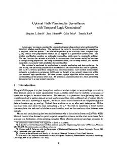
Figure 1: (a) shows the vehicle (marked ”R”) with the obstacle positions shown as black squares. The Green4 dot identifies the goal (b) shows the finite state representation of the possible one-step moves from the current position. (d) shows uncontrollable transitions ”u” from states corresponding to blocked grid locations to ”q⊖ ”
We consider a 2D workspace for the mobile agents. This restriction on workspace dimensionality serves to simplify the exposition and can be easily relaxed. To set up the problem, the 5
the discretized workspace. We specify a particular location as the fixed goal and consider the problem of finding optimal and feasible paths from arbitrary initial grid locations in the workspace. Figure 1(a) illustrates the basic problem setup. We further assume that at any given time instant the robot occupies one particular location (i.e. a particular square in Figure 1(a)). As shown in Figure 1, the robot has eight possible moves from any interior location. The boundaries are handled by removing the moves that take the robot out of the workspace. The possible moves are modeled as controllable transitions between grid locations since the robot can ”choose” to execute a particular move from the available set. We note that the number of possible moves (8 in this case) depends on the chosen fidelity of discretization of the robot motion and also on the intrinsic vehicle dynamics. The complexity results presented in this paper only assumes that the number of available moves is significantly smaller compared to the number of grid squares, i.e., the discretized position states. Specification of inter-grid transitions in this manner allows us to generate a finite state automaton (FSA) description of the navigation problem. Each square in the discretized workspace is modeled as a FSA state with the controllable transitions defining the corresponding state transition map. The formal description of the model is as follows:
Algorithm 1: Computation of Optimal Supervisor input : P, χ, C output: Optimal set of disabled transitions D ⋆ begin Set D [0] = ∅ ; /* Initial disabling set */ e[0] = Π e; Set Π /* Initial event prob. matrix */ Set θ⋆[0] = 0.99, Set k = 1 , Set Terminate = false; while (Terminate == false) do Compute θ⋆[k] ; /* Algorithm 2 */ [k] ⋆ e [k−1] e[k] = 1−θ[k−1] Π ; Set Π 1−θ⋆
Compute ν[k] ; for j = 1 to n do for i = 1 to n do σ [k] Disable all controllable qi − → q j s.t. ν[k] j < νi ; σ
[k] Enable all controllable qi − → q j s.t. ν[k] j ≧ νi ;
Collect all disabled transitions in D [k] ; if D [k] == D [k−1] then Terminate = true; else k = k + 1; D ⋆ = D [k] ;
/* Optimal disabling set */
end
workspace is first discretized into a finite grid and hence the approach developed in this paper falls under the generic category of discrete planning. The underlying theory does not require the grid to be regular; however for the sake of clarity we shall present the formulation under the assumption of a regular grid. The obstacles are represented as blocked-off grid locations in
˜ χ) be a Probabilistic Finite State AuLet GNAV = (Q, Σ, δ, Π, tomaton (PFSA). The state set Q consists of states that correspond to grid locations and one extra state denoted by q⊖ . The necessity of this special state q⊖ is explained in the sequel. The grid squares are numbered in a pre-determined scheme such that each qi ∈ Q \ {q⊖ } denotes a specific square in the discretized workspace. The particular numbering scheme chosen is irrelevant. In the absence of dynamic uncertainties and state estimation errors, the alphabet contains one uncontrollable S event i.e. Σ = ΣC {u} such that ΣC is the set of controllable events corresponding to the possible moves of the robot. The uncontrollable event u is defined from each of the blocked states and leads to q⊖ which is a deadlock state. All other transitions (i.e. moves) are removed from the blocked states. Thus, if a robot moves into a blocked state, it uncontrollably transitions to the deadlock state q⊖ which is physically interpreted to be a collision. We further assume that the robot fails to recover from collisions which is reflected by making q⊖ a deadlock state. We note that q⊖ does not correspond to any physical grid location. The set of blocked grid locations along with the obstacle state q⊖ is denoted as QOBSTACLE j Q. Figure 1 illustrates the navigation automaton for a nine state discretized workspace with two blocked squares. Note that the only outgoing transition from the blocked states q1 and q8 is u. Next we augment the navigation FSA by specifying event generation probabilities defined by the map π˜ : Q × Σ → [0, 1] and the characteristic state-weight vector specified as χ : Q → [−1, 1]. The characteristic state-weight vector [20] assigns scalar weights to the PFSA states to capture the desirability of ending up in each state.
Algorithm 2: Computation of the Critical Lower Bound θ⋆ input : P, χ output: θ⋆ begin Set θ⋆ = 1, Set θcurr = 0; Compute P , M0 , M1 , M2 ; for j = 1 to n do for i = 1 to n� do � if Pχ i − Pχ j , 0 then � � 1 θcurr = 8M2 Pχ i − Pχ j else for r = 0 to n� do � if M0 χ i , M0 χ j then Break; else � � � � if M0 M1r χ , M0 M1r χ then j i Break; if r == 0 then |{(M0 −P)χ}i −{(M0 −P)χ} j | θcurr = ; 8M2 else if r > 0 AND r ≤ n then |( M0 M1 χ)i −( M0 M1 χ) j | θcurr = ; 2r+3 M 2
else θcurr = 1 ; θ⋆ = min(θ⋆ , θcurr ) ; end
Definition 13. The characteristic weights are specified for the 6
navigation automaton as follows: −1 1 χ(qi ) = 0
Notation 2.1. For notational simplicity, we use
if qi ≡ q⊖ if qi is the goal otherwise
νi# (L(qi )) = ν# (qi ) = ν# |i
(3)
where ν# = θmin [I − (1 − θmin )Π# ]−1 χ
In the absence of dynamic constraints and state estimation uncertainties, the robot can ”choose” the particular controllable transition to execute at any grid location. Hence we assume that the probability of generation of controllable events is uniform over the set of moves defined at any particular state.
Definition 16 (ν⋆ -path). A ν⋆ -path ρ(qi , q j ) from state qi ∈ Q to state q j ∈ Q is defined to be an ordered set of PFSA states ρ = {qr1 , · · · , qrM } with qrs ∈ Q, ∀s ∈ {1, · · · , M}, M ≤ C ARD(Q) such that
Definition 14. Since there is no uncontrollable events defined at any of the unblocked states and no controllable events defined at any of the blocked states, we have the following consistent specification of event generation probabilities: ∀qi ∈ Q, σ j ∈ Σ, π˜ (qi , σ j ) =
(
1 , No. of controllable events at qi
1,
(5c)
∀s ∈ {1, · · · , M}, ∀t ≦ s, ν# (qrt ) ≦ ν# (qrs )
(5d)
∀qi ∈ Q \ QOBSTACLE , L(qi ) j ΣC⋆ Corollary 1. (Obstacle Avoidance:) There exists no ν⋆ -path from any unblocked state to any blocked state in the optimally supervised navigation automaton G⋆NAV .
2.4. Decision-theoretic Optimization of PFSA The above-described probabilistic finite state automaton (PFSA) based navigation model allows us to compute optimally feasible path plans via the language-measure-theoretic optimization algorithm [20] described in Section 2. Keeping in line with nomenclature in the path-planning literature, we refer to the language-measure-theoretic algorithm as ν⋆ in the sequel. For the unsupervised model, the robot is free to execute any one of the defined controllable events from any given grid location (See Figure 1(b)). The optimization algorithm selectively disables controllable transitions to ensure that the formal measure vector of the navigation automaton is elementwise maximized. Physically, this implies that the supervised robot is constrained to choose among only the enabled moves at each state such that the probability of collision is minimized with the probability of reaching the goal simultaneously maximized. Although ν⋆ is based on optimization of probabilistic finite state machines, it is shown that an optimal and feasible path plan can be obtained that is executable in a purely deterministic sense. Let GNAV be the unsupervised navigation automaton and G⋆NAV be the optimally supervised PFSA obtained by ν⋆ . We note that νi# is the renormalized measure of the terminating plant G⋆NAV (θmin ) with substochastic event generation probability mae θmin = (1 − θmin )Π. e Denoting the event generating function trix Π (See Definition 3) for G⋆NAV and G⋆NAV (θmin ) as π˜ : Q × Σ → Q and π˜ θmin : Q × Σ → Q respectively, we have
(4b)
(5b)
Proposition 1. For the optimally supervised navigation automaton G⋆NAV , we have
Definition 15. The navigation model id defined to have identical connectivity as far as controllable transitions are concerned implying that every controllable transition or move (i.e. every element of ΣC ) is defined from each of the unblocked states.
∀qi ∈ Q, σ j ∈ Σ, π˜ θmin (qi , σ j ) = (1 − θmin )˜π(qi , σ j )
qrM = q j ∀i, j ∈ {1, · · · , M}, qri , qr j
Lemma 1. There exists an enabled sequence of transitions from state qi ∈ Q \ QOBSTACLE to q j ∈ Q \ {q⊖ } in G⋆NAV if and only if there exists a ν⋆ -path ρ(qi , q j ) in G⋆NAV .
The boundaries are handled by ”surrounding” the workspace with blocked position states shown as ”boundary obstacles” in the upper part of Figure 1(c).
(4a)
(5a)
We reproduce without proof the following key results pertaining to ν⋆ - planning as reported in [18].
if σ j ∈ ΣC otherwise
π˜ θmin (qi , ǫ) = 1
qr1 = qi
Proposition 2 (Existence of ν⋆ -paths). There exists a ν⋆ -path ρ(qi , qGOAL ) from any state qi ∈ Q to the goal qGOAL ∈ Q if and only if ν# (qi ) > 0. Corollary 2. (Absence of Local Maxima:) If there exists a ν⋆ path from qi ∈ Q to q j ∈ Q and a ν⋆ -path from qi to qGOAL then there exists a ν⋆ -path from q j to qGOAL , i.e., � � ^ ∀qi , q j ∈ Q ∃ρ1 (qi , qGOAL ) ∃ρ2 (qi , q j ) ⇒ ∃ρ(q j , qGOAL ) 2.5. Optimal Tradeoff between Computed Path Length & Availability Of Alternate Routes ω1 qj σ1 qi σ2
ω2 ω3 qGOAL
ω4 qk
ν# (q j ) > ν# (qk )
ω
Figure 2: Tradeoff between path-length and robustness under dynamic uncertainty: σ2 ω is the shortest path to qG OAL from qi ; but the ν⋆ plan may be σ1 ω1 due to the availability of larger number of feasible paths through q j .
7
Majority of reported path planning algorithms consider minimization of the computed feasible path length as the sole optimization objective. However, the ν⋆ algorithm can be shown to achieve an optimal trade-off between path lengths and availability of feasible alternate routes. If ω is the shortest path to goal from state qk , then the shortest path from state qi (with σ2 qi −−→ qk ) is given by σ2 ω. However, a larger number of feasiσ1 ble paths may be available from state q j (with qi −−→ q j ) which may result in the optimal ν⋆ plan to be σ1 ω1 . Mathematically, each feasible path from state q j has a positive measure which may sum to be greater than the measure of the single path ω from state qk . The condition ν# (q j ) > ν# (qk ) would then imply that the next state from qi would be computed to be q j and not qk . Physically it can be interpreted that the mobile gent is better off going to q j since the goal remains reachable even if one or more paths become unavailable. The key results [18] are as follows:
We do not need to actually decompose trajectories, it is merely a conceptual construct that gives us a theoretical basis for computing the probabilities of uncontrollable transitions from observed robot dynamics (as described later in Section 5, and therefore incorporate the amortized effect of uncertainties in the navigation automaton. 0
−1
−2 −5.4 −5.6
−3
−5.8 −6 −6.2
−4
Lemma 2. For the optimally supervised navigation automaton G⋆NAV , we have ∀qi ∈ Q \ QOBSTACLE , ∀ω ∈ L(qi ), νi# ({ω}) = θmin
Experimental Run at NRSL with SEGWAY RMP
−6.4 1.4 1.6 1.8
−5
�|ω| � 1−θ min χ(δ# (qi , ω)) C ARD (ΣC )
−6
σ1
Proposition 3. For qi ∈ Q \ QOBSTACLE , let qi −−→ q j → · · · → qGOAL be the shortest path to the goal. If there exists qk ∈ Q \ σ2 QOBSTACLE with qi −−→ qk for some σ2 ∈ ΣC such that ν# (qk ) > ν# (q j ), then the number of distinct paths to goal from state qk is at least C ARD(ΣC ) + 1.
−7 Plan Actual Trajectory −8 0
1
2
3
4
XY Scale in meters
The lower bound computed in Proposition 3 is not tight and if the alternate paths are longer or if there are multiple ’shortest’ paths then the number of alternate routes required is significantly higher. Detailed examples can be easily presented to illustrate situation where ν⋆ opts for a longer but more robust plan.
Figure 3: Plan execution with SEGWAY RMP at NRSL, Pennstate
3.1. The Modified Navigation Automaton e χ) = (Q, Σ, δ, Π, The modified navigation automaton GMOD N AV is defined similar to the formulation in Section 2.3, with the exception that the alphabet Σ is defined as follows:
3. Generalizing The Navigation Automaton To Accommodate Uncertain Execution
Σ = ΣC ∪ ΣUC ∪ {u}
(6)
where ΣC is the set of controllable moves from any unblocked navigation state (as before), while ΣUC is the set of uncontrollable transitions that can occur as an effect of the platform dynamics and oather uncertainty effects. We assume that for each σ ∈ ΣC , we have a corresponding event σu in ΣUC , such that both σ and σu represent the same physical move from a given navigation state; but while σ is controllable and may be disabled, σu is uncontrollable. Although for 2D circular robots we have: C ARD (ΣC ) = C ARD(ΣUC ), in general, there can exist uncontrollable moves reflecting estimation errors that cannot be realized via a single controllable move. For example, for planar rectangular robots with a non-zero minimum turn radius, there can be an uncontrollable shift in the heading without any change in the xy-positional coordinates, which may reflect errors in heading estimation, but such a move cannot be executed via controllable transitions due to the restriction on the minimum turn radius. We will discuss these issues in more details in the sequel.
In this paper, we modify the PFSA-based navigation model to explicitly reflect uncertainties arising from imperfect localization and the dynamic response of the platform to navigation commands. These effects manifest as uncontrollable transitions in the navigation automaton as illustrated in Figure 4. Note, while in absence of uncertainties and dynamic effects, one can disable transitions perfectly, in the modified model, such disabling is only partial. Choosing the probabilities of the uncontrollable transitions correctly allows the model to incorporate physical movement errors and sensing noise in an amortized fashion. A sample run with a SEGWAY RMP at NRSL is shown in Figure 3. Note that the robot is unable to follow the plan exactly due to cellular discretization and dynamic effects. Such effects can be conceptually modeled by decomposing trajectory fragments into sequential combinations of controllable and uncontrollable inter-cellular moves as illustrated in Figure 4(c). 8
F LF L
RF
e8 e1
LF
e2
e7
C
e6
Q, ∀σu ∈ ΣUC implying that γ(GMOD ) = 1, while in pracN AV tice, we expect γ(GMOD ) < 1. N AV
F
e3
R
e7
L
C
RB
• In Definition 17, we allowed for the possibility of π˜ (qi , σu ) being dependent on the particular navigation states qi ∈ Q. A significantly simpler approach would be to redefine the probability of the uncontrollable events π˜ (qi , σu ) as follows: X 1 π˜ (qi , σu ) (8) π˜ AV (σu ) = C ARD(Q) q ∈Q
R
e2 , e3 , e4 , e5 , e6 RB B
e5 e4 LB
RF
e8 e1
LB
B (a)
(b)
F LF
Uncontrollable Move
J4
J0 Controllable Move
Trajectory J7
RF
e e81
e7 e′6
L
i
LB
e′2
C e′5
e′4
e′3
RB
where π˜ AV (σu ) is the average probability of the uncontrollable event σu being generated. (R Partially Disabled
The averaging of the probabilities of uncontrollable transitions is justified in situations where we can assume that the dynamic response of the platform is not dependent on the location of the platform in the workspace. In this simplified case, the event generation probabilities for GMOD can be stated as: ∀qi ∈ Q \ N AV {qGOAL }, σ j ∈ Σ,
B (d)
(c)
π˜ (qi , σ j ) =
Figure 4: (a) shows available moves from the current state (C) in unsupervised navigation automaton. (b) shows the enabled moves in the optimally supervised PFSA with no dynamic uncertainty, (c) illustrates the case with dynamic uncertainty, so that the robot can still uncontrollably (and hence unwillingly) make the disabled transitions, albeit with a small probability, i.e., probability of transitions e′2 , e′3 , e′4 etc. is small. (d) illustrates the concept of using uncontrollable transitions to model dynamical response for a 2D circular robot: J0 is the target cell from J7 , while the actual trajectory of the robot (shown in dotted line) ends up in J4 . We can model this trajectory fragment as first executing a controllable move to J0 and then uncontrollably moving to J4 .
σu ∈ΣUC
Definition 18. The event generation probabilities for GMOD is N AV defined as follows: ∀qi ∈ Q \ {qGOAL }, σ j ∈ Σ, P ˜ i ,σu ) 1− σu ∈ΣUC π(q No. of controllable events at qi , if σ j ∈ ΣC π˜ (qi , σ j ) = π˜ (qi , σ j ), if σ j ∈ ΣUC 1, otherwise
and for the goal, we define as before: ( 1 , π˜ (qGOAL , σ j ) = No. of controllable events at qi 1,
π˜ AV (σ j ), 1,
if σ j ∈ ΣC if σ j ∈ ΣUC otherwise
The key difficulty is allowing the aforementioned dependence on states is not the decision optimization that would follow, but the complexity of identifying the probabilities; averaging results in significant simplification as shown in the sequel. Thus, even if we cannot realistically average out the uncontrollable transition probabilities over the entire state space, we could decompose the workspace to identify subregions where such an assumption is locally valid. In this paper, we do not address formal approaches to such decomposition, and will generally assume that the afore-mentioned averaging is valid throughout the workspace; the explicit identification of the sub-regions is more a matter of implementation specifics, and has little to do with the details of the planning algorithm presented here, and hence will be discussed elsewhere. In Section 5, we will address the computation of the probabilities of uncontrollable transitions from observed dynamics. First, we will establish the main planning algorithm as a solution to the performance optimization of the navigation automaton in the next section.
Definition 17. The coefficient of dynamic deviation γ(GMOD ) is N AV defined as follows: X π˜ (qi , σu ) (7) γ(GMOD ) = 1 − max N AV qi ∈Q
γ(GMOD ) N AV No. of controllable events at qi ,
if σ j ∈ ΣC otherwise
4. Optimal Planning Via Decision Optimization Under Dynamic Effects
Note that we assume there is no uncontrollability at the goal. This assumption is made for technical reasons clarified in the sequel and also to reflect the fact that once we reach the goal, we terminate the mission and hence such effects can be neglected.
The modified model GMOD can be optimized via the measureN AV theoretic technique in a straightforward manner, using the ν⋆ algorithm reported in [18]. The presence of uncontrollable transitions in GMOD poses no problem (as far as the automaton optiN AV mization is concerned), since the underlying measure-theoretic optimization is already capable of handling such effects [20]. However the presence of uncontrollable transitions weakens some of the theoretical results obtained in [18] pertaining to navigation, specifically the absence of local maxima. We show
We note the following: • In the idealized case where we assume platform dynamics is completely absent, we have π˜ (qi , σu ) = 0, ∀qi ∈ 9
that this causes the ν⋆ planner to lose some of its crucial advantages, and therefore must be explicitly addressed via a recursive decomposition of the planning problem.
Proof. Let ℘ be the stationary probability vector for the stochastic transition probability matrix corresponding to the navigation automaton GMOD , for a starting state from which a N AV feasible path to goal exists. (Note that ℘ may depend on the starting state; Figure 5 illustrates one such example. However, once we fix a particular starting state, the stationary vector ℘ is uniquely determined). The selective disabling of controllable events modifies the transition matrix and in effect alters ℘, such that ℘T χ is maximized [20], where χ is the characteristic weight vector, i.e. , χi = χ(qi ). Recalling that χ(qGOAL ) = 1, χ(q⊖) = −1 and χ(qi ) = 0 if qi is neither the goal nor the abstract obstacle state q⊖ , we conclude that the optimization, in effect, maximizes the quantity:
Proposition 4 (Weaker Version of Proposition 2). There exists a ν⋆ -path ρ(qi , qGOAL ) from any state qi ∈ Q to the goal qGOAL ∈ Q if ν# (qi ) > 0. Proof. We note that ν# (qi ) > 0 implies that there necessarily exists at least one string ω of positive measure initiating from qi and hence there exists at least one string that terminates on qGOAL . The proof then follows from the definition of ν⋆ -paths (See Definition 16). Remark 2. Comparing with Proposition 2, we note that the only if part of the result is lost in the modified case.
ψ = ℘GOAL − ℘⊖
(9)
Remark 3. We note that under the modified model, ν# (qi ) < 0 needs to be interpreted somewhat differently. In absence of any dynamic uncertainty, ν# (qi ) < 0 implies that no path to goal exists. However, due to weakening of Proposition 1 (See Proposition 4), ν# (qi ) < 0 implies that the measure of the set of strings reaching the goal is smaller to that of the set of strings hitting an obstacle from the state qi .
Also, note that the optimized navigation automaton has only two dump states, namely the goal qGOAL and the abstract obstacle state q⊖ . That the goal qGOAL is in fact a dump state is ensured by not having uncontrollable transitions at the goal (See Definition 18). Hence we must have
The ν⋆ -planning algorithm is based on several abstract concepts such as the navigation automaton and the formal measure of symbolic strings. It is important to realize that in spite of the somewhat elaborate framework presented here, ν⋆ optimization is free from heuristics, which is often not the case with competing approaches. In this light, the next proposition is critically important as it elucidates this concrete physical connection.
implying that
∀qi ∈ Q \ {qGOAL , q⊖ }, ℘i = 0
(10)
℘GOAL + ℘⊖ = 1 =⇒ ψ = 2℘GOAL − 1 = 1 − 2℘⊖
(11a) (11b)
Hence it follows that the optimization maximizes ℘GOAL and simultaneously minimizes ℘⊖ . Remark 4. It is easy to see that Proposition 5 remains valid if χ(qGOAL ) = χGOAL > 1. In fact, the result remains valid as long as the characteristic weight of the goal is positive and the characteristic weight of the abstract obstacle state q⊖ is negative.
No Connecting Path
Obstacles
4.1. Recursive Problem Decomposition For Maxima Elimination Weakening of Proposition 1 (See Proposition 4) has the crucial consequence that Corollary 2 is no longer valid. Local maxima can occur under the modified model. This is a serious problem for autonomous planning and must be remedied. The problem becomes critically important when applied to solution of mazes; larger the number of obstables, higher is the chance of ending up in a local maxima. While elimination of local maxima is notoriously difficult for potential based planning approaches, ν⋆ can be modified with ease into a recursive scheme that yields maxima-free plans in models with non-zero dynamic effects (i.e. with γ(GMOD ) < 1). N AV It will be shown in the sequel that for successful execution of the algorithm, we may need to assign a larger than unity characteristic weight χGOAL to the goal qGOAL . A sufficient lower bound for χGOAL , with possible dependence on the recursion step, is given in Proposition 6. The basic recursion scheme can be described as follows (Also see the flowchart illustration in Algorithm 3):
A B Goal
Figure 5: Absence of uncontrollable transitions at the goal imply that there is no path in the optimally disabled navigation automaton from point A to point B (or vice versa), since all controllable transitions will necessarily be disabled at the goal. It follows that the stationary probability vector may be different depending on whether one starts left or right to the goal. However, note that that any two points on the same side have a path (possibly made of uncontrollable transitions) between them; implying that the stationary probability vector will be identical if either of them is chosen as the start locations.
Proposition 5. Given that a feasible path exists from the starting state to the goal, the ν⋆ planning algorithm under nontrivial dynamic uncertainty (i.e. with γ(GMOD ) < 1) maximizes N AV the probability ℘GOAL of reaching the goal while simultaneously minimizing the probability ℘⊖ of hitting an obstacle. 10
Proof. Statement 1: We first consider the first recursion step, i.e., the case where k = 0 and Qk = {qGOAL } (See Algorithm 3). We note that the goal qGOAL achieves the maximum measure on account of the fact that only qGOAL has a positive characteristic weight, i.e., we have
1. In the first step (i.e., at recursion step k = 1) we execute ν⋆ -optimization on the given navigation automaton GMOD N AV and obtain the measure vector ν# [k] . 2. We denote the set of states with strictly positive measure as Qk (k denotes the recursion step), i.e., Qk = {qi ∈ Q : ν# [k] |i > 0}
(12)
∀qi ∈ Q, ν# [1] |GOAL ≧ ν# [1] |i
3. If Qk = Qk−1 , the recursion terminates; else we update the characteristic weights as follows: ∀qi ∈ Qk , χ(qi ) = χ[k] G OAL
(15)
It follows that all controllable transitions from the goal will be disabled in the optimized navigation automaton obtained at the end of the first recursion step (See Definition 8 and Algorithms 1 & 2), which in turn implies that the non-renormalized measure of the goal (at the end of the first recursion step) is 1 given by χGOAL θmin . The Hahn Decomposition Theorem [46], allows us to write:
(13)
and continue the recursion by going back to the first step and incrementing the step number k.
ν# |i = ν# (L+ (qi )) + ν# (L− (qi ))
(16)
⋆
Algorithm 3: Flowchart for recursive ν -planning
where L+ (qi ), L− (qi ) are the sets of strings initiating from state qi that have positive and negative measures respectively. Let qi ∈ Q \ {qGOAL } such that qGOAL is reachable from qi in one hop. We note that since it is possible to reach the goal in one hop from qi , we have:
Problem: GMOD N AV 1. Set: ∀qi ∈ Qk χ(qi ) = χ[k] G OAL 2. Eliminate Uncont. transitions from all qi ∈ Qk
Initialize: k = 0, Q0 = {qG OAL } Execute ν⋆
Set k = k + 1
ν# (L+ (qi )) ≧ θmin ×
Define: Qk = {qi ∈ Q : ν# [k] |i > 0} No
Save vector ν# [k]
Qk = Qk−1 ?
Yes Terminate
min
is sufficient to guarantee that the following statements are true: 1. If there exists a state qi ∈ Q \ Qk from which at least one state qℓ ∈ Qk is reachable in one hop, then ν# [k] |i > 0. 2. The recursion terminates in at most C ARD(Q) steps. 3. For the kth recursion step, either Qk % Qk−1 or no feasible path exists to qGOAL from any state qi ∈ Q \ Qk−1 . (1 − θmin ) CARDγ (ΣC )
ν⋆ (q′i ) ≧ −(1 − γ)
qG OAL
(1 − γ)(1 − θmin )
qj
(17)
where the first term arises due to renormalization (See Definition 7), the second term denotes the probability of the transition leading to the goal and the third term is the non-renormalized measure of the goal itself (as argued above). Since it is obvious that the goal achieves the maximum measure, the transition to the goal will obviously be enabled in the optimized automaton, which justifies the second term. It is clear that there are many more strings of positive measure (e.g. arising due to the self loops at the state qi that correspond to the disabled controllable events that do not transition to the goal from qi ) which are not considered in the above inequality (which contributes to making the left hand side even larger); therefore guaranteeing the correctness of the lower bound stated in Eq.(17). Next, we compute a lower bound for ν# (L− (qi )). To that effect, we consider an automaton G′ identical to the navigation automaton at hand in ever respect, but the fact that the qGOAL has zero characteristic. We denote the state corresponding to qi in this hypothesized automaton as q′i , and the set of al states in G′ as Q′ . We claim that, after a measure-theoretic optimization (i.e. after applying Algorithms 1 and 2), the measure of q′i , denoted as ν⋆ (q′i ), satisfies:
[k] Proposition 6. If θmin is the critical termination probability (See Definition 11) for the ν⋆ -optimization in the kth recursion step of Algorithm 3, then the following condition ! C ARD (ΣC ) 1 χ[k] > − 1 (14) G OAL γ 1 − θ[k]
qi
γ(1 − θmin ) χGOAL × C ARD(ΣC ) θmin
(18)
To prove the claim in Eq. (18), we first note that denoting the renormalized measure vector for G′ before any optimization as ν′ , the characteristic vector as χ′ and for any termination probability θ ∈ (0, 1), we have:
1 − θmin q⊖
qk
||ν′ ||∞ = ||θ[I − (1 − θ)Π]−1 χ′ ||∞ ≦ ||θ[I − (1 − θ)Π]−1 ||∞ × 1 = 1 (19)
Figure 6: Illustration for Proposition 6. Uncontrollable events and strings are shown in dashed.
which follows from the following facts: 11
1. For all θ ∈ (0, 1], θ[I − (1 − θ)Π]−1 is a row-stochastic matrix and therefore has unity infinity norm [19] 2. ||χ′ ||∞ = 1, since all entries of χ′ are 0 except for the state corresponding to the obstacle state in the navigation automaton, which has a characteristic of −1.
Qk q j1 σ1 qi
σ
Since the only non-zero characteristic is −1, it follows that no state in G′ can have a positive measure and we conclude from Eq. (19) that: ∀q′j ∈ Q′ , ν(q′j ) ∈ [−1, 0]
(20)
qi
Note that q′i is not blocked itself (since we chose qi such that a feasible 1-hop path to the goal exists from qi ). Next, we subject G′ to the measure-theoretic optimization (See Algorithms 1 & 2), which disables all controllable transitions to the blocked states. In order to compute a lower bound on the optimized measure for the state q′i , (denoted by ν⋆ (q′i ) ), we consider the worst case scenario where all neighboring states that can be reached from q′i in single hops are blocked. Denoting the set of all such neighboring states of qi by N(q′i ), we have: X X ν⋆ (q′i ) = Πuij ν(q′j ) ≧ −1 × Πuij = −1 × (1 − γ) q′j ∈N(q′i )
controllable
qr , where q j ∈ Qk , qr < Qk allows strings which end up in zerocharacteristic states and also (via uncontrollable transitions) on negative-characteristic states. Eq. (25) implies that no enabled string exits Qk . It therefore follows that every string σω starting from the state qi , with ω ∈ ΣC⋆ and δ(qi , σ) ∈ Qk (i.e., σ leads to some state within Qk ) has exactly the same measure as if qi is directly connected to qGOAL and all controllable transitions are disabled at qGOAL (See Figure 7 for an illustration). This conceptual reduction implies that Eq. (17) is valid when Qk % {qGOAL } since the lower bound for ν# (L+ (qi )) can be computed exactly as already done for the case with Qk = {qGOAL }. The argument for obtaining the lower bound for ν# (L− (qi )) is the same as before, thus completing the proof for Statement 1 for all recursion steps of Algorithm 3 . Statement 2: Let QR $ Q be the set of states from which a feasible path to the goal exists. If C ARD (QR ) = 1, then we must have QR = {qGOAL } and the recursion terminates in one step. In general, for the kth recursion step, let C ARD (Qk ) < C ARD (QR ). Since there exists at least one state, not in Qk , from which a feasible path to the goal exists, it follows that there exists at least one state q j from which it is possible to reach a state in Qk in one hop. Using Statement 1, we can then conclude:
(22)
(23)
which after a straightforward calculation yields the bound stated in Eq. 14, and the Statement 1 is proved for the first recursion step, i.e. for Qk = {qGOAL }. To extend the argument to later recursion steps of Algorithm 3, i.e., for k > 0, we argue as follows. Let Qk % {qGOAL } and we have eliminated all uncontrollable transitions from all q j ∈ Qk (as required in Algorithm 3). Further, let qi ∈ Q \ Qk such that it is possible to reach some q j ∈ Q in a single controllable hop, i.e. σ
(25)
which immediately follows from the fact that the optimal configuration (of transitions from states in Qk ) at the end of the ν⋆ -optimization at the kth step would be to have all controllable transitions from states q j ∈ Qk enabled if and only if the transition goes to some state in Qk , since in that case every string initiating from q j terminates on a state having characteristic χGOAL (since there is no uncontrollability from states σ within Qk by construction), whereas if a transition q j −−−−−−−−→
Combining Eqns. (17) and (22), we note that the following condition is sufficient for guaranteeing ν# |i > 0.
controllable
qGOAL
∀q j ∈ Qk , qr < Qk , ν# [k] | j > ν# [k] |r
where Πuij is the probability of the uncontrollable transition from q′i to the neighboring state q′j . Note that we can write Eq. (21) in the worst case scenario where each state in N(q′i ) is blocked, since all controllable transitions from q′i will be disabled in the optimized plant under such a scenario, and only the uncontrollable transitions will remain enabled; and the probabilities of all uncontrollable transitions defined at state qi sums to 1 − γ. It is obvious that the lower bound computed in Eq. (21) also reflects a lower bound for ν# (L− (qi )), since addition of state(s) with positive characteristic or eliminating obstacles cannot possibly make strings more negative. Furthermore, recalling that the goal qGOAL is actually reachable from state qi by a single hop, it follows that not all neighbors of qi in the navigation automaton are blocked, and hence we have the strict inequality:
qi −−−−−−−−→ q j , q j ∈ Qk
σ1 , σ2 σ
We first claim that
(21)
γ(1 − θmin ) × χGOAL > 1 − γ C ARD (ΣC )
q j2
Figure 7: Illustration for Statement 1 of Proposition 6. Note that even if Qk has multiple states, q j1 , q j2 , q j3 , the measure of any string (say σσ1 σ1 σ2 ) from qi is the same as if qi was directly connected to the goal qG OAL with all controllable events disabled at qG OAL . The bottom plate illustrates this by showing the hypothetical scenario where qi is connected to qG OAL by σ and σ1 , σ2 are controllable events disabled at qG OAL . Note that for this argument to work, we must eliminate uncontrollable transitions from all states in Qk .
q′j ∈N(q′i )
ν# (L− (qi )) > −(1 − γ)
q j3
σ1 σ2
(24)
Qk+1 , Qk ⇒ C ARD (Qk+1 ) ≧ C ARD(Qk ) + 1 12
⇒ C ARD(Qk+1 ) ≧ k + 1
(26)
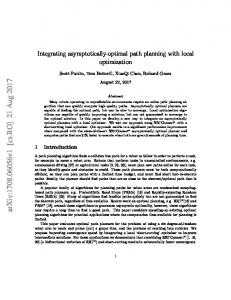
which immediately implies that the recursion must terminate in at most C ARD(Q) steps. Statement 3: Follows immediately from the argument used for proving Statement 2. Remark 5. The generality of Eq. (14) is remarkable. Note that the lower bound is not directly dependent on the exact structure of the navigation automaton; what only matters is the number of controllable moves available at each state, the coefficient of dynamic deviation γ(GMOD ) and the critical termination probN AV ability θmin . Although the exact automaton structure and the probability distribution of the uncontrollable transitions are not directly important, their effect enters, in a somewhat non-trivial fashion, through the value of the critical termination probability. The reader might want to review Algorithm 2 (See also [19, 20]) which computes the critical termination probability in each step of the ν⋆ -optimization for a better elucidation of the aforementioned connection between the structure of the navigation automaton and χGOAL . The dependencies of the acceptable lower bound for χGOAL with the coefficient of dynamic deviation γ(GMOD ), as comN AV puted in Proposition 6, is illustrated in Figures 8(a) and (b). The key points to be noted are: 1. As γ(GMOD ) → 0+ , χGOAL → +∞; which reflects the physN AV ical fact that if no events are controllable, then we cannot optimize the mission plan no matter how large χGOAL is chosen. 2. As γ(GMOD ) → 1, χGOAL → 0; which implies that in the N AV absence of dynamic effects any positive value of χGOAL suffices. This reiterates the result obtained with χGOAL = 1 in [18]. 3. As the number of available controllable moves increases (See Figure 8(a)), we need a larger value of χGOAL ; similarly if the critical termination probability θmin is large, then the value of χGOAL required is also large (See Figure 8(b)). 4. The functional relationships in Figures 8(a) and (b) establish the fact that for relatively smaller number of control) and a small termilable moves, a large value of γ(GMOD N AV nation probability, a constant value of χGOAL = 1 may be sufficient.
Figure 8: Variation of the acceptable lower bound for χG OAL with γ(GMOD ). (a) N AV The set of controllable moves is expanded from C ARD(ΣC ) = 4 to C ARD(ΣC ) = 100 while holding θmin = 0.01 (b) The critical termination probability θmin is varied from 0.001 to 0.1 while holding C ARD(ΣC ) = 8. Note the lines are almost coincident in this case.
the next move, i.e., q j is an acceptable next state if ν# [k] | j > ν# [k] |i and for states qℓ that can be reached from the current state qi via controllable events, we have ν# [k] | j ≧ ν# [k] |ℓ . • if ∀k ∈ {1, · · · , K}, qi < Qk , then terminate operation because there is no feasible path to the goal. • Note that this entails keeping K vectors in memory. 2. (The Assembled Plan Approach:) • Use ν# [k] , k ∈ {1, · · · , K} to obtain the assembled plan vector ν# A following Algorithm 4, which assigns a real value ν# A |i to each state qi in the workspace. We refer to this map as the assembled plan.
4.2. Plan Assembly & Execution Approach The plan vectors ν# [k] (Say, there are K of them, i.e., k ∈ {1, · · · , K}) obtained via the recursive planning algorithm described above, can be used for subsequent mission execution in two rather distinct ways:
• Make use of the gradient defined by ν# A to reach the goal, by sequentially moving to states with increasing values specified by the assembled plan, i.e.,. if the current state is qi ∈ Q, then q j is an acceptable next state if ν# A | j > ν# A |i and for states qℓ that can be reached from the current state qi via controllable events, we have ν# A | j ≧ ν# A |ℓ .
1. (The Direct Approach:) • At any point during execution, if the current state qi ∈ Qk for some k ∈ {1, · · · , K}, then use the gradient defined by the plan vector ν# [k] to decide on 13
since q j ∈ Qk−1 ∧ qi ∈ Qk , it follows from Algorithm 4, that ν# A | j ≧ 1 + ν# A |i > 0. It follows that the same argument can be used recursively to find ν⋆ -paths ρ(q j , qℓ1 ), · · · , ρ(q j , qGOAL ) if and only if ν# A |i > 0. To complete the proof, we still need to show that if there exists a feasible path from a state qi to the goal qGOAL , then there exists a ν⋆ -path ρ(qi , qGOAL ). We argue as follows: Let qi = qr1 → qr2 → · · · → qrm−1 → qrm = qGOAL be a feasible path from the state qi to qGOAL . Furthermore, assume if possible that
Algorithm 4: Assembly of Plan Vectors [k]
1 2 3 4 5 6 7 8 9 10 11 12 13 14 15 16 17
input : ν# , k = 1, · · · , K (Plan Vectors) output: ν# A (Assembled Plan) begin /* Zero vector */ Set ν# A = 0; for k = 1 : K do for i ∈ Q do ν# tmp |i = 0; if ν# [k−1] |i > 0 then tmp ν# |i = 1; else if ν# [k] |i > 0 then tmp ν# |i = ν# [k] |i ; endif endif endfor ν# A = ν# A + ν#tmp; endfor end
∀k ν# [k] |i ≦ 0
(27)
i.e., there exists no ν⋆ -path from qi to qGOAL w.r.t ν# A . We observe that since it is possible to reach qGOAL from qrm−1 in one hop, using Proposition 6 we have: ν# [1] |rm−1 > 0 ⇒ qrm−1 ∈ Q1
(28)
ν# [1] |rm−2 > 0 ⇒ qrm−2 ∈ Q1
(29)
We further note:
[1]
[2]
ν# |rm−2 ≦ 0 ⇒ ν# |rm−2 > 0 ⇒ qrm−2 ∈ Q2
• We show in the sequel that if ν# A |i < 0, then no feasible path exists to the goal.
(30)
Hence, we conclude either qrm−2 ∈ Q2 or qrm−2 ∈ Q1 . It follows by straightforward induction that either q1 ∈ Qm−1 or q1 ∈ Qm−2 , which contradicts the statement in Eq. (27). Therefore, we conclude that if a feasible path to the goal exists from any state qi , then a ν⋆ -path ρ(qi , qGOAL ) (w.r.t ν# A ) exists as well. This completes the proof of Statement 1. Statement 2: Given states qi , q j ∈ Q, assume that we have the ν⋆ -paths ρ1 (qi , qGOAL ) and ρ2 (qi , q j ). We observe that:
Before we can proceed further, we need to formally establish some key properties of the assembled plan approach. In particular, we have the following proposition: Proposition 7. 1. For a state qi ∈ Q, a feasible path to the goal exists from the state qi , if and only if ν# A |i > 0. 2. The assembled plan ν# A is free from local maxima, i.e., if there exists a ν⋆ -path (w.r.t. to ν# A ) from qi ∈ Q to q j ∈ Q and a ν⋆ -path from qi to qGOAL then there exists a ν⋆ -path from q j to qGOAL , i.e., � � ^ ∀qi , q j ∈ Q ∃ρ1 (qi , qGOAL ) ∃ρ2 (qi , q j ) ⇒ ∃ρ(q j , qGOAL )
∃ρ1 (qi , qGOAL ) ⇒ ν# A |i > 0 (See Statement 1) A
A
∃ρ2 (qi , q j ) ⇒ ν# | j ≧ ν# |i (See Definition 16) A
⇒ ν# | j > 0 ⇒ ∃ρ(q j , qGOAL ) (See Statement 1)
3. If a feasible path to the goal exists from the state qi , then the agent can reach the goal optimally by following the gradient of ν# A , where the optimality is to be understood as maximizing the probability of reaching the goal while simultaneously minimizing the probability of hitting an obstacle (i.e. in the sense stated in Proposition 5).
(31a) (31b) (31c)
which proves Statement 2. Statement 3: Statements 1 and 2 guarantee that if a feasible path to the goal exists from a state qi ∈ Q, then an agent can reach the goal by following a ν⋆ -path (w.r.t ν# A ) from qi , i.e., by sequentially moving to states which have a better measure as compared to the current state. We further note that a ν⋆ -path ω w.r.t ν# A from any state qi to qGOAL can be represented as a concatenated sequence ω1 ω2 · · · ωr · · · ωm where ωr is a ν⋆ -path from some intermediate state q j ∈ Q s , for some s ∈ {1, · · · , K}, to some state qℓ ∈ Q s−1 . Since the recursive procedure optimizes all such intermediate plans, and since the outcome “reached goal from qi ” can be visualized as the intersection of the mutually independent outcomes “reached Q s from qi ∈ Q s−1 ”, “reached Q s+1 from q j ∈ Q s ” , · · · , “reached qGOAL from qℓ ∈ Q1 ”, the overall path must be optimal as well. This completes the proof.
Proof. Statement 1: Let the plan vectors obtained by the recursive procedure stated in the previous section be ν# [k] (Say, there are K of them, i.e., k ∈ {1, · · · , K}) and further let the current state qi ∈ Qk for some k ∈ {1, · · · , K}. We observe that on account of Proposition 4, if k = 1, then ν# [k] |i > 0 is sufficient to guarantee that there exists a ν⋆ -path ρ(qi , qGOAL ) w.r.t the plan vector ν# [1] . We further note that ν# [1] |i 0 is also necessary for the existence of ρ(qi , qGOAL ). Extending this argument, we note that, for k > 1, a ν⋆ -path ρ(qi , q j ) with q j ∈ Qk−1 exists (with respect to the plan vector ν# [k] ) if and only if ν# [k] |i > 0. Noting that ν# [k] |i > 0 ⇔ ν# A |i > 0, (See Algorithm 4) we conclude that a ν⋆ -path ρ(qi , q j ) with q j ∈ Qk−1 exists (with respect to the plan vector ν# [k] ) if and only if ν# A |i > 0. Also,
We compute the set of acceptable next states from the following definition. 14
Definition 19. Given the current state qi ∈ Q, Qnext is the set of states satisfying the strict inequality: Qnext = {q j ∈ Q : ν# A | j > ν# A |i }
2. Localization errors: Estimation errors arising from sensor noise, and the limited time available for post-processing exteroceptive data for a moving platform. Even if we assume that the platform is capable of processing sensor data to eventually localize perfectly for a static robot, the fact that we have to get the estimates while the robot pose is changing in real time, implies that the estimates lag the actual robot configuration. Thus, this effect cannot be neglected even for the best case scenario of a 2D robot with an accurate global positioning system (unless the platform speed is sufficiently small).
(32)
We note that Proposition 7 implies that Qnext is empty if and only if the current state is the goal or if no feasible path to the goal exists from the current state. 5. Computation of Amortized Uncertainty Parameters
In our approach, we do not distinguish between the different sources of uncertainty, and attempt to represent the overall amortized effect as uncontrollability in the navigation automaton. The rationale for this approach is straightforward: we visualize actuation errors as the uncontrollable execution of transitions before the controllable planned move can be executed, and for localization errors, we assume that any controllable planned move is followed by an uncontrollable transition to the actual configuration. Smaller is the probability of the uncontrollable transitions in the navigation automaton, i.e., larger is the coefficient of dynamic deviation for each state, smaller is the uncertainty in navigation. From a history of observed dynamics or from prior knowledge, one can compute the distribution of the robot pose around the estimated configuration (in an amortized sense). Then the probability of uncontrollable transitions can be estimated by computing the probabilities with which the robot must move to the neighboring cells to approximate this distribution. The situation for a 2D circular robot is illustrated in Figure 9(a), where we assume that averaging over the observations lead to a distribution with zero mean-error; i.e., the distribution is centered around the estimated location in the configuration space. For more complex scenarios (as we show in the simulated examples), this assumption can be easily relaxed. We call this distribution the deviation contour (D) in the sequel. The amortization or averaging is involved purely in estimating the deviation contour from observed dynamics (or from prior knowledge); a simple methodology for which will be presented in the sequel. However, we first formalize the computation of the uncertainty parameters from a knowledge of the deviation contour. For that purpose, we consider the current state in the navigation automaton to be qi . Recall that qi maps to a set of possible configurations in the workspace. For a 2D circular robot, qi corresponds to a set of x − y coordinates that the robot can occupy, while for a rectangular robot, qi maps to a set of (x, y, θ) coordinates. The footprint of the navigation automaton states in the configuration space can be specified via the map ξ : Q → 2C , where C is the configuration space of the robot. In general, for a given current state qi , we can identify the set N(qi ) ⊂ Q of neighboring states that the robot can transition to in one move. The current state qi is also included in N(qi ) for notational simplicity. In case of the 2D circular robot model considered in this paper, the cardinality of N(qi ) is 8 (provided of course that qi is not blocked and is not a boundary state). For a position s ∈ ξ(qi ) of the robot, we denote a neighborhood of radius r of
Actuation & Localization Uncertainty q1
q8
q2 q8
Q
q7
q3
q7
q1
R
q5
q4
q3
q5
q6 q6
q2
q4
Grid Decomposition
Trajectory (a)
Deviation Contour(D) →
J8
J2
J1
Discretization
B
J1 J8 J7
A
J2 J3
J7
Y
J0
J3
X C
J6
J5
D
J4 J6
J5
J4
(b) Figure 9: (a) Model for 2D circular robot(b) Numerical integration technique for computing the dynamic parameters for the case of a circular robot modele.g. a SEGWAY RMP 200
Specific numerical values of the uncertainty parameters, i.e. the probability of uncontrollable transitions in the navigation automaton can be computed from a knowledge of the average uncertainty in the robot localization and actuation in the configuration space. For simplicity of exposition, we assume a 2D circular robot; however the proposed techniques are applicable to more general scenarios. The complexity of this identification is related to the dynamic model assumed for the platform (e.g. circular robot in a 2D space, rectangular robot with explicit heading in the configuration etc.), the simplifying assumptions made for the possible errors, and the degree of averaging that we are willing to make. Uncertainties arise from two key sources: 1. Actuation errors: Inability of the robot to execute planned motion primitives exactly, primarily due to the dynamic response of the physical platform. 15
the position s in the configuration space as B s,r . The normalized “volume” intersections of B s,r with the footprints of the states included in N(qi ) in the configuration space can be expressed as : R dx Aj , ∀q j ∈ N(qi ) (33) F j (s, r) = Z dx ∪q j A j \ where A j = B s,r ξ(q j ) and dx is the appropriate Lebesgue measure for the continuous configuration space. We observe that the expected or the average probability of the robot deviating to a neighboring state q j ∈ N(qi ) from a location s ∈ ξ(qi ) is given by: Z ∞ F j (s, r)Ddr (34)
these models. Note, in absence of uncertainty, the 4D implementation is superfluous; (x previous , y previous , xcurrent , ycurrent ) has no more information than (xcurrent , ycurrent ) in that case. 15◦
Available Controllable → Transitions Uncontrollable Move
Figure 10: A rectangular robot unable to execute zero-radius turns. There exists uncontrollable transitions that alter heading in place, which reflects uncertainties in heading estimation, although there are no controllable moves that can achieve this transition
0
Hence, the probability Πuc i j of uncontrollably transitioning to a neighboring state q j from the current state qi is obtained by considering the integrated effect of all possible positions of the robot within ξ(qi ), i.e. we have: Z Z ∞ F j (s, r)Ddrds ξ(qi ) 0 Z Z (35) = Πuc ∞ ij X F j (s, r)Ddrds q j ∈N(qi )
ξ(qi )
Controllable Move
Next, we present a methodology for computing the relevant uncertainty parameters as a function of the robot dynamics. We assume a modular plan execution framework, in which the lowlevel continuous controller on-board the robotic platform is sequentially given a target cell (neighboring to the current cell) to go to, as it executes the plan. The robot may be able to reach the cell and subsequently receives the next target, or may end up in a different cell due to dynamic constraints, when it receives the next target from this deviated cell as dictated by the computed plan. The inherent dynamical response of the particular robot determines how well the patform is able to stick to the plan. We formulate a framework to compute the probabilities of uncontrollable transitions that best describe these deviations.
0
where dr, ds are appropriate Lebesgue measures on the continuous configuration space of the robot. It is important to note that the above formulation is completely general and makes no assumption on the structure of the configuration space, e.g., the calculations can be carried out for 2D circular robots, rectangular robots or platforms with more complex kinematic constraints equally well. Figures 13(a)-(c) illustrate the computation for a circular robot with eight controllable moves, .e.g., the situation for a SEGWAY RMP. The 2D circular case is however the simplest, where any state that can be reached by an uncontrollable transition, can also be reached by a controllable move. For more complex scenarios, this may not be the case. For example, in the rectangular model, with constraints on minimum turn radius, the robot may not be able to move via a controllable transition from (x, y, h1) to (x, y, h2 ), where hi , i = 1, 2 is the heading in the initial and final configurations. However, there most likely will be an uncontrollable transition that causes this change, reflecting uncertainty in the heading estimation (See Figure 10). Also, one can reduce the averaging effect by considering more complex navigation automata. For example, for a 2D circular robot, the configuration state can be defined to be (x previous , y previous , xcurrent , ycurrent ), i.e. essentially considering a 4D problem. The identification of the uncertainty parameters on such a model will capture the differences in the uncontrollable transition probabilities arising from arriving at a given state from different directions. While the 2D model averages out the differences, the 4D model will make it explicit in the specification of the navigation automaton (See Figure 15). In the sequel, we will present comparative simulation results for
Definition 20. The raw deviation ∆R (t) as a function of the operation time t is defined as follows: ∆R (t) = Θ(p(t), ζ(t))
(36)
where p(t) is the current location of the robot in the workspace coordinates, ζ(t) is the location of the point within the current target cell which is nearest to the robot position p(t) (See Figure 11), and Θ(·, ·) is an appropriate distance metric in the configuration space. The robot will obviously take some time to reach the target cell, assuming it is actually able to do so. We wish to eliminate the effect of this delay from our calculations, since a platform that is able to sequentially reach each target cell, albeit with some delay, does not need the plan to be modified. Furthermore, unless velocity states are incorporated in the navigation automata, the plan cannot be improved for reducing this delay. We note that the raw deviation ∆R (t) incorporates the effect of this possibly variable delay and needs to be corrected for. We do so by introducing the delay corrected deviation ∆(t) as follows: Definition 21. The delayed deviation ∆d (t, η) is defined as: ∆d (t, η) = Θ(p(t + η(t)), ζ(t)) 16
(37)
J2
J1
Since the delay may vary slowly, the computed value of η⋆ may vary from one observation interval to another. For each interval Ik ∈ {I1 , · · · , I M }, one can obtain the approximate probability distribution of the delay corrected deviation ∆(t), which is denoted as D[k] . Therefore, from a computational point of view, D[k] is just a histogram constructed from the ∆(t) values for the interval Ik (for a set of appropriately chosen histogram bins or intervals). For a sufficiently large number of observation intervals {I1 , · · · , I M }, one can capture the deviation dynamics of the robotic platform by computing the expected distribution of ∆(t), i.e. computing D, which can be estimated simply by:
J3
J4 Target Cell ∆R (t) J0
J5
J8 ∆R (t0 )
J6 J7
D=
S
Current Location (time = t0 )
Robot Trajectory
J2
C
J3
J4
σuTarget Cell B σu
J5
J0
J6
6. Summarizing ν⋆ Planning & Subsequent Execution J8
The complete approach is summarized in Algorithm 5. The planning and plan assembly steps (Lines 2 & 3) are to be done either offline or from time to time when deemed necessary in the course of mission execution. Replanning may be necessary if the dynamic model changes either due to change in the environment or due to variation in the operational parameters of the robot itself, e.g., unforeseen faults that alter or restrict the kinematic or dynamic degrees of freedom. Onwards from Line 4 in Algorithm 5 is the set of instructions needed for mission execution. Line 5 computes the set of states to which the robot can possibly move from the current state. We select one state from the set of possible next states which have a strictly higher measure compared to the current state in the computed plan. It is possible that the set of such states Qnext (See Line 6) has more than one entry. Choice of any element in Qnext as the next desired state is optimal in the sense of Proposition 5 . However, one may use some additional criteria to aid this choice to yield plans suited to the application at hand, e.g., to minimize change of current direction of travel. For example one may choose the state from Qnext that requires least deviation from the current direction of movement, to minimize control effort. In general, we can penalize turning using a specified penalty β ∈ [0, 1] as follows:
A D
J7 S
Current Location (time = t0 )
(41)
Once the distribution for the delay corrected deviation has been computed, we can proceed to estimate the probabilities of the uncontrollable transitions, as described before. Determination of the uncertainty parameters in the navigation model then allows us to use the proposed optimization to compute optimal plans which the robot can execute. We summarize the sequential steps in the next section.
(a)
J1
M 1 X [k] D M k=1
Robot Trajectory
(b) Figure 11: Illustration for computation of amortized dynamic uncertainty parameters
where η(t) is some delay function satisfying ∀τ ∈ R, η(τ) ≥ 0. Definition 22. The delay corrected deviation ∆(t) as a function of the operation time t is defined as: ∆ (t, η) (38) ∀t ∈ R, ∆(t) = argin f ∆d (t, η) : ∀τ ∈ R, η(τ) ≥ 0
d
Note that Definition 22 incorporates the possibility that the delay may vary in the course of mission execution. We will make the assumption that although the delay may vary, it does so slowly enough to be approximated as a constant function over relatively short intervals. If we further assume that we can make observations only at discrete intervals, we can approximately compute ∆(t) over a short interval I = [tinit , t f inal ] as follows: Θ(p(t + η), ζ(t)) ∀t ∈ I, ∆(t) = argmin (39)
Definition 23. Given a turning penalty β ∈ [0, 1], the turn penalized measure values on the set of possible next states Qnext is computed as follows:
Θ(p(t+η),ζ(t)):η∈N∪{0}
Furthermore, the approximately constant average delay η⋆ over the interval I can be expressed as: η⋆ = argmin Θ(p(t + η), ζ(t)) (40)
∀q ∈ Qnext , νβ (q) = (1 − β)ν# A (q) + β cos(h(q))
(42)
where h(q) is the heading correction required for transitioning to q ∈ Qnext , which for 2D circular robots is calculated as the
η∈N∪{0}
17
gamma = 0.98
5 10
X: 8 Y: 15
gamma = 0.98
5 10
X: 8 Y: 15
gamma = 0.98
5 10
X: 8 Y: 15
10
15
15
15
15
20
20
20
20
25
25
25
25
30
30
30
30
35
35
35
35
40
40
40
40
45
45
45
45
50
5
10
15 (a) β = 0
20
25
50
5
10
15
20
25
50
(b) β = 0.35
5
10
15
20
gamma = 0.98
5
25
50
(c) β = 0.75
X: 8 Y: 15
5
10
15
20
25
(d) β = 1
Figure 12: Effect of increasing turning penalty β on making turns in choice of local transitions post ν⋆ -optimization. Note that the potential gradient is identical in all four cases. The start state is (8, 15) as shown. The gradient shown (by the arrows) is for the computed measure vector ν# A , and hence is identical for all four cases
a non-positive measure (due to uncertainties and execution errors), then execution is terminated and the mission is declared unfeasible from that point (See Line 14). It is important to note that if a particular configuration maps to a navigation state with non-positive measure, then no feasible path to goal exists from that configuration, irrespective of uncertainty effects. This underscores the property of the proposed algorithm that it finds optimal feasible paths; even if the only feasible path is very unsafe, it still is the only feasible path; and is therefore the optimal course of action (See Proposition 7 Statement 3).
angular correction between the line joining the center of the current state to that of q, and the line joining the center of the last state with that of the current one. the direction of the last state. The robot then chooses qnext as the state q ∈ Qnext which has the maximum value for νβ (q). The effect of penalizing turns is shown in the Figure 12. Note that for maximum turn penalty, the computed plan is almost completely free from kinks. Also, note that the ν⋆ optimization ensures that all these plans have the same probability of success and collision. As stated in Line 8, the robot may not be successful to actually transition to the next chosen state due to dynamic effects. In particular, if the state that the robot actually ends up in has
7. Verification & Validation
Algorithm 5: Summarized Planning & Mission Execution 1 2 3 4 5 6 7 8 9 10 11 12 13 14 15 16 17 18
In this section we validate the proposed planning algorithm via detailed high fidelity simulation studies and in experimental runs on a heavily instrumented SEGWAY RMP 200 at the robotic testbed at the Networked Robotics & Systems Laboratory (NRSL), Pennstate. The results of these experiments adequately verify the theoretical formulations and the key claims made in the preceding sections.
input : Model GMOD N AV begin /* ←− Planning & Plan Assembly −→ */; Compute decomposed plans ν# [k] ; /* Algorithm 3 */ Compute assembled plan ν# A ; /* Algorithm 4 */ /* ←− Mission Execution −→ */; while true do � σ Find set of neighbors: N(qi ) = q ∈ Q : ∃σ ∈ ΣC s.t. qi − →q; � A A Compute Qnext = q j ∈ N(qi ) : ∀qk ∈ N(qi ), ν# | j > ν# |k ; Choose one state qnext from set Qnext ; Attempt to move to qnext ; /* May be unsuccessful */ Read current state qi ; /* Possibly qi , qnext */ if qi == qG OAL then Mission Successful Terminate Loop; else if ν# A |i ≦ 0 then Mission Failed Terminate Loop; endif endif endw end
Remark 6. In depicting simulation results in the sequel, we refer to “computed paths/plans”. It is important to clarify, what we mean by such a computed or simulated path. The computed path is the sequence of configuration states that the robot would enter, if the uncertainties do not force it to deviate, i.e., the path depicts the best case scenario under the uncertainty model. Thus, the depictions merely give us a feel for the kind of paths the robot would take; in actual implementation, the trajectories would differ between runs. Also, when we refer to lengths of the computed paths, we are referring to the lengths of the paths in the best case scenario, i.e., the tight lower bound on the path length that will actually be encountered. 18
19 0.3 0.2
18
0.1 0 0 0.05 0.3
η⋆
Run 1
0.1 0.15
0.2 0.25
.003
17 5
10 15 Run Number
20
25
0.5
Run 2
γ= .93
.015
16 0
0.3 0.35
.015
.003
.003
.015
.015
.003
0.2
0.4
0.1 0.2 0.25
0.3 0.35
0.3 0.2
0.2 0.25
0.3 0.35
Deviation ∆
0.1 0 16
17 η⋆
(a)
18
19
Probability
0.1 0.15
0.4 0.3 Run 3 0.2 0.1 0 0 0.05 0.1 0.15
Probability
Probability
0 0 0.05
0.4 0.35 0.3 0.25 0.2 0.15 0.1 0.05 0 0 0.05 0.1 0.15 0.2 0.25 0.3 0.35 ∆ (c)
(b)
Figure 13: Computation of dynamic uncertainty parameters from observed dynamics for SEGWAY RMP 200 at NRSL, Pennstate: (a) shows the observed distribution D of the deviation ∆ for different runs, (b) shows the distribution of the delay η⋆ for the various runs, Lower plate in (c) illustrates the expected distribution E(D) for deviation ∆ while the upper plate in (c) enumerates the probabilities of the uncontrollable transitions to the neighboring cells, and the coefficient of dynamic ) deviation γ(GMOD N AV
5
5
5
10
10
10
15
15
15
20
20
20
25
25
25
30
30
30
35
35
35
40
40
40
45
45
45
50
5
10
15
20
(a) γ(GMOD )=1 N AV
25
50
5
10
20
15
(b) γ(GMOD ) = 0.98 N AV
25
50
5
10
15
20
25
(c) γ(GMOD ) = 0.9 N AV
Figure 14: Simulation results with a circular robot model and different values of the coefficient of dynamic deviation γ(GMOD ). Note the response of the navigation N AV ) is decreased. gradient as γ(GMOD N AV
7.1. Simulation Results for Circular Robots The recursive version of the modified ν⋆ planning algorithm presented in this paper (See Algorithm 5) is first validated in a detailed simulation example as illustrated in Figures 13(a-c) and 14(a-c). The workspace is chosen to be a 50 × 30 grid, with obstacles placed at shaded locations, as illustrated. The size of the workspace is chosen to correspond with the size of the actual test-bed, where experimental runs on the robotic platform would be performed subsequently. Plates (a)-(c) in Figure 14 illustrates the gradient of the optimized measure vector (by short arrows) and a sample optimal path from location (15, 10) (up-
per,left) to the goal (40, 20) (down,right). We note that the “potential field” defined by the measure gradient converges (i.e. has an unique sink) at the goal. Also, note that the coefficient of dynamic deviation γ(GMOD ) is decreased, the algorithm responds N AV by altering the optimal route to the goal. In particular, the optimal path for smaller values of γ(GMOD ) stay further away from N AV the obstacles. The key point to note here is that the the proposed algorithm guarantees that this lengthening of the route to account for dynamic uncertainty is optimal, i.e., further lengthening by staying even further from the obstacles yields no advantage in a probabilistic sense. This point has a direct practical 19
implication; one that can be verified experimentally as follows. Let us assume that we have a real-world robot equipped with on-board reactive collision avoidance, by which we can ensure that the platform does not actually collide with obstacles under dynamic uncertainty, but executes corrections dictated by local reactive avoidance. Then, the preceding result would imply that a using the correct value of dynamic deviation (for the specific platform) in the planning algorithm would result in routes that require the least number of local corrections; which in turn ensures minimum time route traversals on the average. It is important to note that the assumption of a circular robot poses no critical restrictions. Similar results can be obtained for more complex models as well, i.e. rectangular platform with constrained turn radius. However, extension to multi-body motion planning would require addressing the algorithmic complexity issues that become important even for the recursive ν⋆ for very large configuration spaces, and is a topic of future work.
Figure 15: Non-symmetric deviation contours arising from explicit dependence on the last discrete position for the robot INIT
GOAL
No uncertainty
7.2. Simulation Results for Non-symmetric Uncertainty As stated in the course of the theoretical development, it is possible to choose the degree of amortization or averaging that one is willing to allow in the specification of the navigation automaton. As a specific example, one may choose to compute the probabilities of uncontrollable transitions with respect to some length of trajectory history; the simplest case is using the previous state information to yield non-symmetric deviation contours (See Figure 15). The particular type of deviation contours illustrated in Figure 15 is obtained if the platform has a large stopping distance and inertia, and the heading and positional estimates are more or less accurate, i.e., the uncontrollability in the model is a stronger function of the dynamic response, rather than the estimation errors. A typical scenario is the SEGWAY RMP 200 with good global positioning capability, in which factoring in the dynamic response is important due to the invertedpendulum two-wheel kinematics. For this simulation, we use a navigation automaton obtained from discretizing an essentially 4D underlying continuous configuration space. Each state (except the obstacle state) in the navigation automaton maps to a discretized pair of locations, reflecting the current robot location and the one from which it transitioned to the current location. We call this the 4D Model to distinguish it from the the significantly smaller and simpler 2D model. Note that the 2D model can be obtained from the 4D model by merging states with the same current location via averaging the probabilities of uncontrollable transitions over all possible previous states. Also note that (as stated earlier), in the absence of uncertainty, the 4D formulation adds nothing new; explicitly encoding the previous location in the automaton state gives us no new information. Table 1 enumerates the comparative model sizes.
4D model 2D model
Figure 16: Comparative pathlengths for the chosen initial and goal configurations: 65 steps for 2D model, 51 steps for 4D model, 36 steps for the case with no uncertainty
Comparisons of computed plans for a particular set of initial and goal configurations is shown in Figure 16. To accentuate the differences in the computed plans, the deviation contours were chosen so that the probability of uncontrollable transition in the current direction of travel is significantly more compared to that of deviating to left or right, i.e., the contours are really narrow ellipses. Under such a scenario, the platform is more capable of navigating narrow corridors as compared to the amortized 2D counterpart. This is reflected in the paths shown in Figure 16, where the path for the 4D model is shorter, and goes through some of the narrow bottlenecks, while the path for the 2D model takes a safer path. Note, the path for the nouncertainty case is even more aggressive, and shorter. In practical implementation, when the uncontrollable probabilities are identified from observed dynamics or pre-existing continuous models, the differences in the two cases are often significantly less.
Table 1: Comparison of 4D and 2D Models
2D Model 4D Model
Map Size 40 × 40 40 × 40
No. of States 1600 256 × 104
Alphabet Size 8 8
7.3. Simulation Results for Rectangular Robots The proposed planning algorithm is next applied to the case of rectangular robots, specifically ones that have a minimum non-zero turn radius. We further impose the constraint that the 20
platform cannot travel backwards, which is a good assumption for robots that have no ranging devices in the rear, and also for aerial vehicles (UAVs). Even assuming planar operation, this problem is essentially 3D, with the navigation automaton reflecting the underlying configuration states of the form (x, y, h) where h is the current heading, which can no longer be neglected due to the inability of the patform to turn in place. A visual comparison of the models for the circular and rectangular cases is shown in Figure 17(e). The heading is discretized at 15◦ intervals, implying we have 24 discrete headings. This also means that for the same planar workspace, the number of states in the rectangular model is about 24 times larger the number of states for the circular model. Also, while in the circular case, we had 8 neighbors, the number of neighboring configurations increases to 8 × 24 + 24 = 216 However, not all neighbors can be reached via controllable transitions due to the restriction on the turn radius; we assume a maximum turn of ±45◦ in the model considered for the simulation. As explained earlier, all the neighbors may be reachable via uncontrollable transitions, which reflects uncertainties in estimation (See Figure 10). We test the algorithm with different values of γ(GMOD ) as ilN AV lustrated in Figure 17(a-d). Note the trajectories become more rounded and less aggressive (as expected) as the uncertainty is increased. Also note that the heading at the goal is different for the different cases. This is because, in the model , we specified as goals any state that maps to the goal location in the planar grid irrespective of the heading, i.e., the problem was solved with essentially 24 goals. Although for simplicity, the theoretical development was presented assuming a single goal, the results can be trivially shown to extend to such scenarios. The trajectories however, will be significantly different if we insist on having a particular heading at the goal (See Figure 18). In the simulations for the rectangular model, we deliberately assume that any neighbor that cannot be reached via a controlled move is not reachable by an uncontrollable transition as well. Although this is not what we expect to encounter in field, the purpose of this assumption is to bring out an interesting consequence that we illustrate in Figures 19(a-b). As explained above, this assumption implies that we have little or no uncertainty in local heading estimations (since the robot cannot turn in place, so there is no uncontrollable transition that alters heading in place). It therefore follows, that under this scenario, the platform would find it relatively safe to navigate narrow passages. This is exactly what we see in Figure 19(b), where the circular robot with same coefficient of dynamic uncertainty, really goes out of way to avoid the narrow passage, while the rectangular robot goes through.
there are two opposing effects in play here; while a longer path that stays away from the obstacles influences to decrease the collision probability, the very fact that the path is longer has an increasing influence arising from the increased probability that an uncontrollable sequence would execute from some point in the path that leads to a collision. At relatively high values of γ(GMOD ), the first effect dominates and we can effectively deN AV crease the collision probability by staying away from the obstacles thereby increasing the path length. However, at low values of γ(GMOD ), the latter effect dominates, implying that N AV increased path lengths are no longer advantageous. This interesting phenomenon is illustrated in Figure 20(b), where we clearly see that the path lengths peak in the γ(GMOD ) = 0.72 N AV to γ(GMOD ) = 0.85 range (for the maze considered in FigN AV ure 20(a)). Also note that the configuration space has to be sufficiently complex to actually see this effect; which is why we do not see this phenomenon in the simulation results presented in Figures 14(a-c). 7.5. Experimental Runs on SEGWAY RMP 200 The proposed algorithm is validated on a SEGWAY RMP 200 which is a two-wheeled robot with significant dynamic uncertainty. In particular, the inverted-pendulum dynamics prevents the platform from halting instantaneously, and making sharp turns at higher velocities. At low velocities, however, the platform can make zero radius turns. The global positional fix is provided via an (in-house developed) over-head multi-camera vision system, which identifies the position and orientation of the robot in the testbed. The vision system yields a positional accuracy of ±7.5 cm, and a heading accuracy or ±0.1 rad for a stationary robot. The accuracy deteriorates significantly for a mobile target, but noise correction is intentionally not applied to simulate a high noise uncertain work environment. Furthermore, the cameras communicate over a shared wireless network and randomly suffers from communication delays from time to time, leading to delayed positional updates to the platform. In the experimental runs conducted at NRSL the workspace discretized into a 53 × 29 grid. Each grid location is about 4 sq. ft. allowing the SEGWAY to fit completely inside each such discretized positional state which justifies the simplified circular robot modeling. The runs are illustrated in Figure 22. The robot was run at various allowed top speeds (vmax ) ranging from 0.5 mph to over 2.25 mph. Only the extreme cases are illustrated in the figure. For each speed, the uncertainty parameters were estimated using the formulation presented in Section 5. The sequence of computational steps for the low velocity case (vmax = 0.5 mph) are shown in Figure 13. Note the coefficient of dynamic deviation for the low velocity case turns out to be γlow = 0.973. For the high velocity case, (vmax = 2.25 mph), the coefficient is computed to have a value of γhigh = 0.93 (calculation not shown). Also, the robot is equipped with an on-board low-level reactive collision avoidance algorithm, which ensures that the platform does not actually collide due path deviations; but executes local reactive corrections when faced with such situations. The platform is equipped with multiple high frequency sonars, infra-red range finders and a high-precision SICK LMS
7.4. Simulation Results for Mazes We simulate planning in a maze of randomly placed static obstacles. A sample case with optimal paths computed for different coefficients of dynamic deviation is illustrated in Figure 20(a). A key point to note is that the optimal path is lengthens first as γ(GMOD ) is decreased, and then starts shortening N AV again, which may seem paradoxical at first sight. However, this is exactly what we expect. Recall that the proposed algorithm minimizes the probability of collision. Also note that 21
0
0
5
5
10
10
15
15
20
20
25
25 30
25
20
15
10
5
0
30
25
)=1 (a) γ(GMOD N AV
20
15
10
5
0
5
0
) = 0.8 (b) γ(GMOD N AV
0
0
5
5
10
10
15
15
20
20
25
25 30
25
20 (c)
15
) γ(GMOD N AV
10
5
0
30
25
= 0.5
20 (d)
15◦
15
) γ(GMOD N AV
10 = 0.1
Discretized Neighboring Configurations
Rectangular Model
Circular Model (e)
Figure 17: Comparative trajectories for rectangular model
200 laser range finder. The data from these multiple ranging devices, mounted at various key locations on the platform, must be fused to obtain correct situational awareness. In this paper, we skip the details of this on-board information processing for the sake of brevity. The overall scheme is illustrated in Figure 21
ments of 0.1. The expectation is that using the correct coefficient of dynamic deviation (as computed above for the two chosen speeds) for the given speed, would result in the minimum number of local corrections, leading to minimum average traversal times over thirty laps. The results are summarized in plates (c) (for the low velocity case) and (f) (for the high velocity case) in Figure 22. Note the fitted curve in both cases attain the minimal point very close to the corresponding computed γ values, namely, 0.97 for vmax = 0.5 mph and 0.92 for vmax = 2.25 mph. A visual comparison of the trajectories in the plates (a) and (d) clearly reveal that the path execution has significantly more uncertainties
In the experimental runs, we choose two waypoints (marked A and B) in Figure 22 (plates a,b,d,e), and the mission is to plan and execute the optimal routes in sequence from A to B, back to A and repeat the sequence a specified number of times (thirty). This particular mission is executed for each top speed for a range of γ values, namely with γ ∈ [0.75, 1] with incre22
Goal Location
Goal Location Goal Heading Note Difference
Note Difference
(a) Strict Goal Heading Requirement
(b) No Heading Requirement
) = 0.8: Case (a) we demand that the robot reach the goal with a specified heading (−150◦ ). Figure 18: Comparative trajectories for rectangular model for γ(GMOD N AV Case (b): Any heading at the goal is acceptable
Circular Robot
Note
Note
)=1 (a) γ(GMOD N AV
Rectangular Robot
) = 0.8 (b) γ(GMOD N AV
Figure 19: Comparative trajectories for rectangular model and circular model to illustrate the effect of different uncertainty assumptions: (a) Trajectories in the absence of uncertainty (b) Trajectories with γ(GMOD ) = 0.8. N AV
in the high velocity case. Also note, that the higher average speed leads to repeated loss of position fix information in locations around (row = 20, column = 35). Plates (b) and (e) illustrate the sequence of waypoints invoked by the robot in the two cases, being the centers of the states in the navigation automaton that the robot visits during mission execution. Note that in the high velocity case, the variance of the trajectories is higher leading to a larger set of waypoints been invoked. Note that three distinct zones (denoted as Zone A, Zone B and Zone C) can be identified in the plates (e) and (f) of Figure 22. Zone A reflects the operation when γ is (incorrectly assumed to be) too large, leading to too many corrections, and hence execution time can be reduced by reducing γ. In Zone B, reducing γ increases execution time, since now the trajectories becomes unnecessarily safe, i.e. stays away from obstacles way more than necessary leading to longer than required paths and hence increased execution time. Zone C represents a sort of saturation zone where reducing γ has no significant effect, arising from the fact that the paths cannot be made arbitrarily safe by increasing
path lengths. Although the experimental runs were not done for smaller values of γ, we can say from the experience with maze simulations (See Section 7.4), that the execution times will start reducing again as γ is further reduced. These results clearly show that the approach presented in this paper successfully integrates amortized dynamical uncertainty with autonomous planning, and establishes a computationally efficient framework to cyber-physical motion planning. 8. Summary & Future Research The recently proposed PFSA-based path planning algorithm ν⋆ is generalized to handle amortized dynamic uncertainties in plan execution, arising from the physical limitations of sensing and actuation, and the inherent dynamic response of the physical platforms. The key to this generalization is the introduction of uncontrollable transitions in the modified navigation automaton, and showing that ν⋆ can be implemented in a recursive fashion to guarantee plan optimality under such circumstances. 23
G 120 0.8
110 100 0.1 1
90 Path Lengths
0.4
80
60 0.1
S
Simulated Data Polynomial Fit
70 0.2
0.3
0.4
0.5
0.6
0.7
0.8
0.9
1
) γ(GMOD N AV (b)
(a)
Figure 20: Effect of dynamic uncertainty on the optimal path lengths computed by ν⋆ . Plate (a) illustrates the optimal paths for γ(GMOD ) = 1.0, 0.8, 0.4, 0.1 from N AV ) for the maze the start location marked by S and the goal marked by G. Plate (b) illustrates the variation of the length of the optimal paths as a function of γ(GMOD N AV illustrated in (a).
the whole problem at once; however care must be taken to ensure that the computed solution is not too far from the optimal one. One the areas of current research is an algorithmic decomposition of the configuration space such that individual blocks are solved in parallel on communicating processors, with the interprocessor communication ensuring close-to-global optimality. We envision such an approach to be ideaally suited to scenarios involving multiple agents distributed over a large workspace which cooperatively solve the global planning problem in an efficient resource-constrained manner. 3. Handling partially observable dynamic events: In this paper all uncontrollable transitions are assumed to be perfectly observable. Physical errors and onboard sensor failures may need to be modeled as unobservable transitions and will be addressed in future publications. A generalization of the measure-theoretic optimization technique under partial observation has been already reported [48]. The future goal in this direction is to incorporate the modifications to allow ν⋆ handle loss of observation and feedback information.
Figure 21: Autonomous navigation scheme with ν⋆ implementation on heavily instrumented Segway RMP (shown in inset).
The theoretical algorithmic results is verified in detailed highfidelity simulations and subsequently validated in experimental runs on the SEGWAY RMP 200 at NRSL, Pennstate. 8.1. Future Work Future work will extend the language-measure theoretic planning algorithm to address the following problems: 1. Multi-robot coordinated planning: Run-time complexity grows exponentially with the number of agents if one attempts to solve the full Cartesian product problem. However ν⋆ can be potentially used to plan individually followed by an intelligent assembly of the plans to take interaction into account. 2. Hierarchical implementation to handle very large workspaces: Large workspaces can be solved more efficiently if planning is done when needed rather than solving
References [1] J.-C. Latombe, Robot Motion Planning, International Series in Engineering and Computer Science; Robotics: Vision, Manipulation and Sensors, Kluwer Academic Publishers, Boston, MA, U.S.A., 1991, 651 pages. [2] S. M. LaValle, Planning Algorithms, Cambridge University Press, Cambridge, U.K., 2006, available at http://planning.cs.uiuc.edu/. [3] K. Kondo, Motion planning with six degrees of freedom by multistrategicbidirectional heuristic free-space enumeration, IEEE Transactions on Robotics and Automation 7 (3) (1991) 267–277.
24
45 A
45 A
45 A
45 A
40
40
40
40
35
35
35
35
30
30
30
30
25
25
25
25
20
20
20
20
15
15
15
15
10
10
10
B 5
10
10
B 15
20
25 5
B
10
15
(a)
20
25
5
20
25 5
Zone A
165
195
Zone C
160 Time (sec)
Zone C Zone B 0.91
) γ(GMOD N AV
0.93
0.95
0.97
0.99
15
20
25
Mean Runtime Smooth Spline
170
185
10
(d)
175
Mean Runtime Smooth Spline
200
Time (sec)
15 (c)
205
180
10
(b)
210
190
B
Zone A Zone B
155 150 145
0.75
0.8
γ(GMOD ) N AV
0.85
0.9
0.95
(f)
(e)
Figure 22: Experimental runs on SEGWAY RMP 200: (a)-(c) Low speed runs and (d)-(f) High speed runs: Plates (a) and (d) shows the trace of the robot positions as read by the overhead vision system at NRSL for the low and high speed runs respectively. (b) and (e) shows the waypoints invoked by the robot in course of executing the specified mission in the low and high speed cases respectively. Plates (c) and (f) illustrate the variation of the mean mission execution times with the coefficient of dynamic deviation used fro planning in the low and high speed cases respectively.
[4] J. Borenstein, Y. Koren, The vector field histogram-fast obstacle avoidance for mobiledoi:DOI:10.1016/j.robot.2009.07.028. robots, Robotics and Automation, IEEE Transactions on 7 (3) (2002) 278–288. [11] J. R. Andrews, N. Hogan, Impedance Control as a Framework for Imdoi:10.1109/70.88137. plementing Obstacle Avoidance in a Manipulator, ASME, Boston, MA, URL http://dx.doi.org/10.1109/70.88137 1983, pp. 243–251. [5] T. Lozano-Perez, A simple motion-planning algorithm for general robot [12] O. Khatib, Real-time obstacle avoidance for manipulators and mobile manipulators, IEEE Transactions on Robotics and Automation 3 (3) robots, in: IEEE International Conference on Robotics and Automation, (1987) 224–238. Vol. 2, St. Louis, MI, 1985, pp. 500–505. [6] D. A. Anisi, J. Hamberg, X. Hu, Nearly time-optimal paths for a ground [13] B. H. Krogh, A generalized potential field approach to obstacle avoidvehicle, Journal of Control Theory and Applications. ance control, in: International Robotics Research Conference, Bethlehem, [7] J. Barraquand, B. Langlois, J.-C. Latombe, Robot motion planning with 1984. many degrees of freedom and dynamic constraints, MIT Press, Cam[14] M. Kumar, D. Garg, R. Zachery, Multiple mobile agents control via artifibridge, MA, USA, 1990. cial potential functions and random motion, in: Proceedings of the ASME [8] J. Langelaan, Tree-based trajectory planning to exploit atmospheric enInternational Mechanical Engineering Congress and Exposition, ASME, ergy, in: American Control Conference, 2008, 2008, pp. 2328–2333. Seattle, WA, 2007. doi:PaperNo.IMECE2007-41521. [15] S. Sarkar, E. Halland, M. Kumar, Mobile robot path plandoi:10.1109/ACC.2008.4586839. ning using support vector machines, in: ASME Dynamic Sys[9] S. Lahouar, E. Ottaviano, S. Zeghoul, L. Romdhane, M. Ceccatems and Control Conference, ASME, Ann Arbor, Michigan, 2008. relli, Collision free path-planning for cable-driven parallel robots, doi:PaperNo.DSCC2008-2200. Robotics and Autonomous Systems 57 (11) (2009) 1083 – 1093. [16] J. Borenstein, Y. Koren, Potential field methods and their inherent limdoi:DOI:10.1016/j.robot.2009.07.006. itations for mobile robot navigation, in: Proceedings of the 1991 IEEE [10] L. M. Ortega, A. J. Rueda, F. R. Feito, A solution to the International Conference on Robotics and Automation, 1991, pp. 1398– path planning problem using angle preprocessing, Robotics 1404. and Autonomous Systems In Press, Corrected Proof (2009) –.
25
[17] R. Tilove, Local obstacle avoidance for mobile robots based on the method of artificial potentials, Robotics and Automation, 1990. Proceedings., 1990 IEEE International Conference on (1990) 566–571 vol.1doi:10.1109/ROBOT.1990.126041. [18] I. Chattopadhyay, G. Mallapragada, A. Ray, ν⋆ : a robot path planning algorithm based on renormalized measure of probabilistic regular languages, International Journal of Control 82 (5) (2008) 849–867. [19] I. Chattopadhyay, A. Ray, Renormalized measure of regular languages, Int. J. Control 79 (9) (2006) 1107–1117. [20] I. Chattopadhyay, A. Ray, Language-measure-theoretic optimal control of probabilistic finite-state systems, Int. J. Control. [21] J. M. O’kane, B. Tovar, P. Cheng, S. M. Lavalle, Algorithms for planning under uncertainty in prediction and sensing, in: Chapter 18 in Autonomous Mobile Robots: Sensing, Control, Decision-Making, and Applications, Marcel Dekker, 2005, pp. 501–547. [22] T. Lozano-Perez, M. T. Mason, R. H. Taylor, Automatic Synthesis of Fine-Motion Strategies for Robots, The International Journal of Robotics Research 3 (1) (1984) 3–24. doi:10.1177/027836498400300101. [23] A. Lazanas, J. Latombe, Landmark-based robot navigation, Vol. 92, AAAI Press, San Jose, California, 1992, pp. 816–822. [24] T. Fraichard, R. Mermond, Path planning with uncertainty for car- like robots, in Proc. of the IEEE Intl. conf. on Robotics & Automation (1998) 27–32. [25] N. J. Nilsson, Principles of Artificial Intelligence, Tioga, 1980. [26] H. Takeda, J.-C. Latombe, Sensory uncertainty field for mobile robot navigation, in Proc. of the IEEE Intl. conf. on Robotics & Automation (1992) 2465–2472. [27] P. E. Trahanias, Y. Komninos, Robot motion planning: Multi- sensory uncertainty fields enhanced with obstacle avoidance, in: Proc. of the IEEE/RSJ Intl. conf. on Intelligent Robots and Systems, 1996. [28] N. A. Vlassis, P. Tsanakas, A sensory uncertainty field model for unknown and non-stationary mobile robot environments, in: Proceedings of the IEEE Intl. conf. on Robotics & Automation, 1998. [29] N. Roy, S. Thrun, Coastal navigation with mobile robots, in: Advances in Neural Information Processing, Systems (NIPS, 1999. [30] R. Alami, T. Simeon, Planning robust motion strategies for a mobile robot, in: Proc. of the IEEE Intl. conf. on Robotics & Automation, 1994. [31] B. Bouilly, T. Simeon, R. Alami, A numerical technique for plan- ning motion strategies of a mobile robot in presence of uncertainty, in: Proc. of the IEEE Intl. conf. on Robotics & Automation, 1995. [32] M. Khatib, B. Bouilly, T. Simeon, R. Chatila, Indoor navigation with uncertainty using sensor-based motions, in Proc. of the IEEE Intl. conf. on Robotics & Automation 4 (1997) 3379–3384. [33] J. Barraquand, P. Ferbach, Motion planning with uncertainty: The information space approach, in: Proc. of the IEEE Intl. conf. on Robotics &
Automation, 1995. [34] L. A. Page, A. C. Sanderson, Robot motion planning for sensor-based control with uncertainties, Vol. 2, Nagoya, Japan, 1995, pp. 1333–1340. [35] L. Blackmore, H. Li, B. Williams, A probabilistic approach to optimal robust path planning with obstacles, in: Proceedings of the AIAA Guidance, Navigation and Control ConferenceNavigation and Control Conference, 2006. [36] L. Blackmore, A probabilistic particle control approach to optimal, robust predictive control, in: Proceedings of the AIAA Guidance, Navigation and Control ConferenceNavigation and Control Conference, 2006. [37] A. Lambert, N. L. Fort-Piat, Safe task planning integrating uncertainties and local maps federations, International Journal of Robotics Research, volume 19 (2000) 597–611. [38] A. Lambert, D. Gruyer, Safe path planning in an uncertain-configuration space, in: Robotics and Automation, 2003. Proceedings. ICRA ’03. IEEE International Conference on, Vol. 3, 2003, pp. 4185–4190. doi:10.1109/ROBOT.2003.1242246. [39] J. P. Gonzalez, A. T. Stentz, Planning with uncertainty in position: An optimal and efficient planner, in Proc. of the IEEE/RSJ Intl. conf. on Intelligent Robots and Systems (2005) 2435–2442. [40] J. P. Gonzalez, A. Stentz, Planning with uncertainty in position using high-resolution maps, in: Proc, of the IEEE Intl. conf. on Robotics & Automation, Rome, Italy, 2007. [41] R. Alterovitz, T. Sim´eon, K. Y. Goldberg, The stochastic motion roadmap: A sampling framework for planning with markov motion uncertainty, in: Robotics: Science and Systems, 2007. [42] P. Singla, T. Singh, A novel coordinate transformation for obstacle avoidance and optimal trajectory planning, in: 2008 AAS/AIAA Astrodynamics Specialist Conference and Exhibit, 2008. [43] A. Ray, Signed real measure of regular languages for discrete-event supervisory control, Int. J. Control 78 (12) (2005) 949–967. [44] V. Garg, An algebraic approach to modeling probabilistic discrete event systems, Proceedings of 1992 IEEE Conference on Decision and Control (Tucson, AZ, December 1992) 2348–2353. [45] V. Garg, Probabilistic lnaguages for modeling of DEDs, Proceedings of 1992 IEEE Conference on Information and Sciences (Princeton, NJ, March 1992) 198–203. [46] W. Rudin, Real and Complex Analysis, 3rd ed., McGraw Hill, New York, 1988. [47] I. Chattopadhyay, Quantitative control of probabilistic discrete event systems, PhD Dissertation, Dept. of Mech. Engg. Pennsylvania State University, http:// etda.libraries.psu.edu / theses / approved / WorldWideIndex / ETD-1443. [48] I. Chattopadhyay, A. Ray, Optimal control of infinite horizon partially observable decision processes modeled as generatorsof probabilistic regular languages, International Journal of Control In Press.
26