Formal verification of an interior point algorithm instanciation

Formal verification of an interior point algorithm instanciation Guillaume Davy∗‡ , Eric Feron† , Pierre-Loic Garoche∗ , and Didier Henrion‡

arXiv:1801.03833v1 [cs.LO] 11 Jan 2018

∗

Onera - The French Aerospace Lab, Toulouse, FRANCE ‡ CNRS LAAS, Toulouse, FRANCE † Georgia Institute of Technology, Atlanta GA, USA

Abstract. With the increasing power of computers, real-time algorithms tends to become more complex and therefore require better guarantees of safety. Among algorithms sustaining autonomous embedded systems, model predictive control (MPC) is now used to compute online trajectories, for example in the SpaceX rocket landing. The core components of these algorithms, such as the convex optimization function, will then have to be certified at some point. This paper focuses specifically on that problem and presents a method to formally prove a primal linear programming implementation. We explain how to write and annotate the code with Hoare triples in a way that eases their automatic proof. The proof process itself is performed with the WP-plugin of Frama-C and only relies on SMT solvers. Combined with a framework producing all together both the embedded code and its annotations, this work would permit to certify advanced autonomous functions relying on online optimization.

1

Introduction

The increasing power of computers, makes possible the use of complex numerical methods in real time within cyber-physical systems. These algorithms, despite having been studied for a long time, raise new issues when used online. Among these algorithms, we are concerned specifically with numerical optimization which is used in model predictive control (MPC) for example, by SpaceX to perform computation of trajectory for rocket landing [1]. These iterative algorithms perform complex math operations in a loop until they reach an -close optimal value. This implies some uncertainty on the number of iterations required but also on the reliability of the computed result. We address both these issues in this paper. As a first step, we focus on linear programming, with the long-term objective of proving more general convex optimization problems. We therefore chose to study an interior point algorithm (IPM, Interior Point Method) instead of the famous simplex methods. As a matter of fact simplex is bound to linear constraints while IPMs can address more general convex cones such as the Lorentz cone problems (quadratic programming QP and second-order cone programming SOCP), or Semi-Definite Programming (SDP).

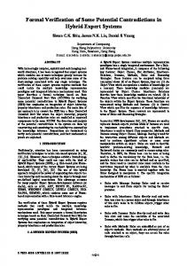
To give the best possible guarantee, we rely on formal methods to prove the algorithm soundness. More specifically we use Hoare Logic[2,3] to express what we expect from the algorithm and rely on Weakest Precondition[4] approach to prove that the code satisfy Fig. 1. Complete toolchain we are interested in, this article focus on writing C code and annotation them. Figure 1 sketches our fully automatic process which, when provided with a convex problem with some unknown values, generates the code, the associated annotation and prove it automatically. We are not going to present all the process in this paper but concentrate on how to write the embedded code, annotate it and automatize its proof. In this first work, we focus on the algorithm itself assuming a real semantics for float variables and leave the floating point problem for future work. However the algorithm itself is expressed in C with all the associated hassle and complexity. We proved the absence of runtime error, the functionality of the code and its termination. This paper is structured as follow. In Section 2 we present some key notions for both convex optimization and formal proof of our algorithm. In Section 3 we present the code structure supporting the later proof process. In Section 4 we introduce our code annotatations. Section 5 focuses on the proof process. Section 6 presents some experimental results.

2

Preliminaries

In order to support the following analyses, we introduce the notions and notations used throughout the paper. First, we discuss Linear Programming (LP) problems and a primal IPM algorithm to solve it. Then, we introduce the reader to Hoare logic based reasoning. 2.1

Optimization

Linear Programming is a class of optimization problems. A linear program is defined by a matrix A of size m × n, and two vectors b, c of respective size m, and n. Definition 1 (Linear program) Let us consider A ∈ Rm×n , b ∈ Rm and c ∈ Rn . We define P (A, b, c) as the linear program: min

x∈Rn ,Ax≤b

hc, xi with hc, xi = cT x

(1)

Definition 2 (Linear program solution) Let us consider the problem P (A, b, c) and assume that an optimal point x∗ exists and is unique. We have then the following definitions: Ef ={x ∈ Rn | Ax ≤ b} f (x) =hc, xi ∗

x = arg min f x∈Ef

(feasible set of P )

(2)

(cost function)

(3)

(optimal point)

(4)

Primal interior point algorithm. We decided to use interior point method (IPM) to enable the future extension of this work to more advanced convex programs. We chose a primal algorithm for its simplicity compared to primal/dual algorithms and we followed Nesterov’s book [5, chap. 4] for the theory. The following definitions present the key ingredients of IPM algorithms: barrier function, central path, Newton steps and approximate centering condition. Fig. 2. Barrier function Barrier function. Computing the extrema, i.e. minimum or maximum, of a function without additional constraints, could be done by analyzing the zeros of its gradiants. However this does not apply in presence of constraints. An approach that amounts to introducing a penalty function F : Ef → R to represent the feasible set, ie. the acceptable region. This function must tend towards infinity when x approaches the border of Ef , cf. Figure 2 for a logarithmic barrier function encoding a set of linear constraints.

Definition 3 The adjusted cost function is a linear combination of the previous objective function f and the barrier function F . f˜(x, t) = t × f (x) + F (x) with t ∈ R (5) The variable t balances the impact of the barrier: when t = 0, f˜(x, t) is independent from the objective while when t → +∞, f˜(x, t) is equivalent to t × f (x). Central path. We are interested in the values of x minimizing f˜ when t varies from 0 to +∞. These values for x characterize a path, the central path: Definition 4 (Central path and analytic center) x ∗ : R+ t

→ Ef 7→ arg min f˜(x, t)

(6)

x∈Ef

x∗ (0) is called the analytic center, it is independent from the cost function.

The central path has an interesting property when t increases: Property 1 lim x∗ (t) = x∗

(7)

t→+∞

The algorithm prerforms a sequence of iterations, updating a point X that follows the central path and eventually reaches the optimal point. At the beginning of an iteration, there exists a real t such that X = x∗ (t). Then t is increased by dt > 0 and x∗ (t+dt) is the new point X. This translation dX is performed by a Newton step as sketched in Fig. 3. One step along the central path Figure 3. Newton step. The Newton’s method computes an approximation of a root of a function G : Rk → Rl . It is a first order method, ie. it relies on the gradient of the function and, from a point in the domain of the neighbourhood of a root, performs a sequence of iterations, called Newton steps. Figure 4 illustrates one of such step. Definition 5 A Newton step transforms Yn into Yn+1 as follows: Fig. 4. Newton step for k =
−1 l=1 Yn+1 − Yn = − G0 (Yn ) G(Yn ) (8) We apply the Newton step to the gradient of f˜, computing its root which coincides with the minimum of f˜. We obtain dX = − F 00 (X)


−1

((t + dt)c + F 0 (X))

(9)

Self-concordant barrier. The convergence of the Newton method is guaranted only in the neighbourhood to the function root. This neighbourhood is called the region of quadratic convergence; this region evolves on each iteration since t varies. To guarantee that the iterate X remains in the region after each iteration, we require the barrier function to be self-concordant: Definition 6 (Self-concordant barrier) A closed convex function g is a νself-concordant barrier if 3

D3 g(x)[u, u, u] ≤ 2(uT g 00 (x)u) 4

(10)

g 0 (x)T g 00 (x)g 0 (x) < ν

(11)

and

From now on we assume that F is a self-concordant barrier. Thus F 00 is non-degenerate([5, Th4.1.3]) and we can define: Definition 7 (Local-norm) kyk∗x =

q y T × F 00 (x)−1 × y

(12)

This local-norm allows to define the Approximate Centering Condition(ACC), the crucial property which guarantees that X remains in the region of quadratic convergence: Definition 8 (ACC) Let x ∈ Ef and t ∈ R+ , ACC(x, t, β) is a predicate defined by kf˜0 (x)k∗x = ktc + F 0 (x)k∗x ≤ β (13) In the following, we choose a specific value for β, as defined in (14). √ 3− 5 (14) β< 2 The only step remaining is the computation of the largest dt such that X remains in the region of quadratic convergence around x∗ (t + dt). dt =

γ kck∗x

(15)

with γ a constant. This choice maintains the ACC at each iteration([5, Th4.2.8]): Theorem 1 (ACC preserved) If we have ACC(X, t, β) and γ ≤ then we also have ACC(X + dX, t + dt, β).

√ β √ 1+ β

−β

For this work, we use the classic self-concordant barrier for linear program: m P F (x) = −log(bi − Ai × x) with A1 , An the columns of A. i=0

Importance of the analytic center. x∗F is required to initiate the algorithm. In case of offline use the value could be precomputed and validated. However in case of online use, its computation itself has to be proved. Fortunatly this can be done by a similiar algorithm with comparable proofs. 2.2

Formal methods

For the same program, different semantics can be used to specify its behavior: (i) a denotational semantics, expressing the program as a mathematical function, (ii) an operational semantics, expressing it as a sequence of basic computations, or (iii) an axiomatic semantics. In the latter case, the semantics can be defined in an incomplete way, as a set of projective statements, i.e. observations. This idea was formalized by Floyd [3], Hoare [6] as a way to specify the expected behavior, the specification, of a program through pre- and post-condition, or assume-guarantee contracts.

Definition 9 (Hoare Triple) Let C : M → M be a program with M the set of its possible memories. Let P and Q, two predicates on M. We say that the Hoare triple {P } C {Q} is valid when ∀m ∈ M, P (m) ⇒ Q(C(m))

(16)

– P is called a precondition or requires and Q the postcondition or ensures. – If C is a function, {P } C {Q} is called a contract. These Hoare triples can be used to annotate programs written in C. In the following, we rely on the ANSI C Specification Language (ACSL)[7], the specification language of Frama-C, to annotate functions. The Frama-C tool processes the annotation language, identifying each Hoare Triple and converting them into logical formulas, using the Weakest Precondition strategy. Definition 10 (Weakest Precondition) The Weakest Precondition of a program c and a postcondition Q is a formula WP(C, Q) such that: 1. {WP(C, Q)} C {Q} is a valid Hoare triple 2. For all P , {P } C {Q} valid implies P ⇒ WP(C, Q) Theorem 2 (Proving Hoare Triple)

WP(C, Q) = R P ⇒R {P } C {Q}

The WP property can be computed mechanically, propagating back the postcondition along the program instructions. An example of such rules is given in Figure 5. The only exception is the while loop rule which requires to be provided with an invariant, this rule is presented later in the document in Figure. 12. Assignement

Sequence

Conditional

WP(x = E, Q) = ∀y, y = E ⇒ Q[x ← y]

WP(S2, Q) = O WP(S1, O) = R WP(S1;S2, Q) = R

WP(S1, Q) = P1 WP(S2, Q) = P2 WP(if (E) S1 else S2, Q) = E ⇒ P1 ∧ ¬E ⇒ P2 Fig. 5. Examples of WP rules

Automation The use of SMT solvers enables the automatic proof of some programs and their annotations. This is however only feasible for properties that could be solved without the need of proof assistant. This requires to write both programs (cf. Section 3) and annotations (cf. Section 4) with some considerations for the proof process.

3

Writing Provable Code

In order to ease the proof process we write the algorithm code in a very specific manner. In the current section we present our modeling choices: we made all variables global, split the code into small meaningfull functions for matrix operations, and transform the while loop into a for loop to address the termination issue. Variables. One of the difficulties when analyzing C code are memory related issues. Two different pointers can reference the same part of the stack. A fine and complex modeling of the memory in the predicate encoding, such as separation logic[8] could address these issues. Another more pragmatic approach amounts to substitute all local variables and function arguments with global static variables. Two static arrays can’t overlap since their memory is allocated at compile time. Since we are targetting embedded system, static variables will also permit to compute and reduce memory footprints. However there are two major drawbacks: the code is a less readable and variables are accessible from any function. These two points usually lead the programmer to mistakes but could be accepted in case of code generation. We tag all variables with the function they belong to by prefixing each variable with its function name. This brings traceability. Function. Proving large functions is usually hard with SMT-based reasonR⇒Q {P } C {R} ing since the generated goals are too Function call WP(f(), Q) = P complex to be discharged automatically. A more efficient approach is to with void f() { C } associate small pieces of code with local contracts, These intermediate anFig. 6. WP rules used for function call notations act as cut-rules in the proof process. The Figure 6 presents the function call used in the WP algorithm. Let A = B[C] be a piece of code containing C. Replacing C by a call to f() { C } requires either to inline the call or to write a new contract {P } f() {Q}, characterizing two smaller goals instead of a larger one. Specifically in the proof of a B[f()], C has been replaced by P and Q which is simpler than a WP computation. Therefore instead of having one large function, our code is structured into several functions: one per basic operation. Each associated contract focuses on a really specific element of the proof without interference with the others. Thereby formulas sent to SMT solvers are smaller and the code is modular. Matrix operation. This is extremely useful for matrix operations. In C, a M × N Matrix operations is written as M × N scalar operation affecting an array representing the resulting matrix. With our methods these operations are gathered in a function annotated by the logic representation of the matrix operation, cf Figure 7. Contracts associated to this small function associate high-level matrix operation to the C low-level computation, acting as refinement contracts.

The encoding hides low-level op-   erations to the rest of the code, lead- /*@ ensures MatVar(dX, 2, 1) ==\old(mat_scal(MatVar(cholesky, 2, 1), -1.0)); ing to two kinds of goals : @ assigns *(dX+(0..2)); */ – Low level operation (memory and basic matrix operation). – High level operation (mathematics on matrices). The structure of the final code after the split in small functions is shown in Figure 8.

void set_dX() { dX[0] = -cholesky[0]; dX[1] = -cholesky[1]; }

Fig. 7. Example of matrix operation: dx %= -cholesky encapsulated in a function for dx and cholesky of size 2 × 1

– compute fill X with the the analytic center and call pathfollowing. – pathfollowing contains the main loop which udpate dX and dt. – compute_pre compute Hessian and gradiant of F which are required for dt and dX. – udpate_dX and udpate_dt call the associated subfunction and update the corresponding value. – compute_dt performs (15), it requires to call Chowlesky to compute the local norm of c. – compute_dX performs (9), Chowlesky is used to inverse the hessian matrix.

Fig. 8. Call tree of the implementation(rose boxes are matrix computation)

While-loop. The interior point algorithm is iterative: it performs the same operation until reaching the stop condition. This stopping criteria depends on the desired precision : (1 + β)β 1 (1 + ) (17)  1−β Proving the termination amounts to find a suitable bound guaranting the obtention of a converged value. We present here the convergence proof of [5] and use it to ensure termination. It relies on the use of the following geometric progression: tk ≥ tstop =

Definition 11 Lower(k) =

γ k−1 γ(1 − 2β) (1 + ) (1 − β)kck∗x∗ 1+β F

(18)

This sequence minimizes t for each iteration k of the algorithm([5, Th4.2.9]): Theorem 3 For all k ∈ N∗ , tk ≥ Lower(k)

(19)

Combined with (17), a maximal number of iteration called klast can be computed: Theorem 4 (Required number of iterations) ln(1 +

(β+1)∗β 1−β )

klast = 1 +

γ∗(1−2β) ) − ln() − ln( (1−β)∗kck ∗ ∗

ln(1 +

x

γ β+1 )

F

(20)

Since we have a termination proof based on the number of iterations, the while-loop can be soundly replaced by a for-loop with klast iterations. As shown in Figure 9, the number of iterations is greater than the one obtained with original while-loop with the stopping criteria but it permits to have absolute guarantee on termination. Analytic center kck∗x∗ is required to Fig. 9. Evolution of t and Lower with the F compute klast , therefore a worst case algorithm, notice that t remains always execution time can be computed if greater than Lower and only if kck∗x∗ has a lower bound F at compilation time.

4

Annotate the code

The code is prepared to ease its proof but the specification still remains to be formalized as function contracts, describing the computation of an -optimal solution. This requires to enrich ACSL with some new mathematics definitions. We introduce a set of axiomatic definition to specify optimization related properties. These definitions require, in turn, additional concepts related to matrices. Similar approaches were already proposed [9] but were too specfic to ellipsoid problems. We present here both the main annotation and the function local contracts, which ease the global proof. Matrix axiomatic. To write the mathematics property, we need to be able to express the notion of Matrix and operations over it. Therefore we defined a new ACSL axiomatic. An ACSL axiomatic permits the specifier to extend the ACSL language with new types and operators, acting as an algebraic specification.

  axiomatic matrix { type LMat;

First, we defined the new type: LMat standing for Logic Matrix. This type is abstract therefore it will be defined by its operators. // Getters logic integer getM(LMat A); logic integer getN(LMat A); logic real mat_get(LMat A, integer i, integer j); // Constructors logic LMat MatVar(double* ar, integer m, integer n) reads ar[0..(m*n)]; logic LMat MatCst_1_1(real x0); logic LMat MatCst_2_3(real x0, real x1, real x2, real x3, real x4, real x5);

Getters allow to extract information from the type while constructors bind new LMat object. The first constructor is followed by a read clause stating which part of the memory affects the corresponding LMat object. The Constant constructor take directly the element of the matrix as argument, it can be replaced with an ACSL array for bigger matrix sizes. logic logic logic logic ...

LMat LMat LMat LMat

mat_add(LMat A, LMat B); mat_mult(LMat A, LMat B); transpose(LMat A); inv(LMat A);

Then the theory defined the operations on the LMat type. These are defined axiomatically, with numerous axioms to cover their various behavior. We only give here a excerpt from that library. axiom getM_add: \forall LMat A, B; getM(mat_add(A, B))==getM(A); axiom mat_eq_def: \forall LMat A, B; (getM(A)==getM(B))==> (getN(A)==getN(A))==> (\forall integer i, j; 0 dot(c, y) >= sol(A, b, c); axiom sol_greater: \forall LMat A, b, c; \forall Real y; (\forall LMat x; mat_gt(mat_mult(A, x), b) ==> dot(c, x) >= y) ==> sol(A, b, c) >= y;

Then we defined some operators representing definitions 7, 8 and 11.

logic real norm(LMat x0, LMat x1, LMat x2, LMat x3) = \sqrt(mat_get(mat_mult(transpose(x2), mat_mult(inv(hess(x0, x1, x3)), x2)), (0), (0))); logic boolean acc(LMat x0, LMat x1, LMat x2, real x3, LMat x4, real x5) = ((norm(x0, x1, mat_add(grad(x0, x1, x4), mat_scal(x2, x3)), x4)) lower(l);*/ (int l = 0; l < NBR;l++) { ... }

Proving the initialization is straighfoward, thanks to the main preconditions. The first invariant preservation is stated by [5, Th4.1.5] which was translated into an ACSL lemma, the second by Theorem 1 and the third one by Theorem 3. The last two loop invariants are combined to prove the second postcondition of pathfollowing thanks to Theorem 5 and NBR equals klast (20).

Theorem 5 [5, Th4.2.7] Let t ≥ 0, and X such that ACC(X, t, β) then cT X − cT X ∗
\old(t)*(1 + void update_t();

N)==hess(A, b, MatVar(X, N, 1)); MatVar(X, N, 1), BETA); MatVar(X, N, 1), BETA + GAMMA); GAMMA/(1 + BETA));*/

The first postcondition is an intermediary results stating that: ACC(X, t + dt, β + γ)

(22)

This result is used as precondition for update_x. The second precondition corresponds to the product of t by the common ratio of the geometric progression Lower, cf. Definition 11 which will be used to prove the second invariant of the loop. The first precondition is a postcondition from update_pre and the second one is the first loop invariant.

5

Automatic proof with SMT solvers.

For each annotated piece of code, the Frama-C WP plugin computes the Weakest precondition and generates all the first order formulas required to validate the Hoare triples. There are two main solutions to prove goals: proving them thanks to a proof assistant – this requires to be done by a human –, or proving them with a fully automatic SMT solver. We decided to rely only on SMT solvers in order to be able to completely automatize the process. Therefore it is better to have lots of small goals instead of several larger ones. We splited the code for this reason and we now split the proof of lemmas into several intermediate lemmas. For example, in order to prove (22) we wrote update_t_ensures1 where P1 is ACC(X, t, β) γ and P2 is dt = kck ∗ x

∀x, t, dt; P1 ⇒ P2 ⇒ ACC(X, t + dt, β)

(update_t_ensures1)

which itself need update_t_ensures1_l0 ∀x, t, dt; P1 ⇒ P2 ⇒ kF 0 (X) + c(t + dt)k∗x ≤ β + γ (update_t_ensures1_l0) Equation update_t_ensures1_l0 needs 3 lemmas to be proven:

∀x, t, dt; P2 ⇒ kc × dtk∗x = γ

(update_t_ensures1_l3)

∀x, t, dt; P1 ⇒ kF 0 (X) + c × tk∗x ≤ β

(update_t_ensures1_l2)

∀x, t, dt; P1 ⇒ P2 ⇒ kF 0 (X) + c(t + dt)k∗x ≤ kF 0 (X) + c × t)k∗x + kc × dtk∗x (update_t_ensures1_l1) The proof tree for the first ensures of update_t can be found in Figure 13.

Fig. 13. Proof tree for (22)(In green proven goal, in white axioms)

6

Experimentations

Frama-C is a powerful tool but not always built for our specific needs therefore we had to do some tricks to make it prove our goals. Using multiple files Frama-C automatically adds, for each goal, all the lemmas as hypotheses. This increases significantely the size of the goal. To avoid this issue that prevented some proofs, we wrote each function or lemma in a separate file. In this file we add as axioms all the lemmas required to prove the goal. This allows us to prove each goal independently with a minimal context. The impact of the separation into multiple function(Section 3) and the separation into multiple files is shown in Table 1. The annotated code can be retrieved from https://github.com/davyg/ proved_primal

7

Related work

Related works include first activities related to the validation of numerical intensive control algorithms. This article is an extension of Wang et al [10] which was presenting annotations for a convex optimization algorithm, namely IMP, but the process was both manual and theoretical: the code annotated within Matlab and without machine checked proofs. An other work from the same authors [9]

2×5

Size of A

4 × 15

8 × 63

Experiences

exp1

exp2

exp3

exp1

exp2

exp3

exp1

exp2

exp3

nb function

1

12

12

1

26

26

1

78

78

nb file

1

1

12

1

1

26

1

1

78

nb proven goal

21

48

48

43

97

97

12

257

264

nb goal

25

48

48

46

97

97

109

264

264

Table 1. Proof results for compute_dt with one function and one file(exp1), with multiple function(exp2) or with multiple file(exp3) and a Timeout of 30s for Alt-Ergo for random generated problem of specific sizes.

presented a similar method than ours but limited to simple control algorithms, linear controllers. The required theories in ACSL were both different and less general than the ones we are proposing here. Concerning soundness of convex optimization, Cimini and Bemporad [11] presents a termination proof for a quadratic program but without any concerns for the proof of the implementation itself. A similar criticism applies to Tøndel, Johansen and Bemporad [12] where another possible approach to online linear programming is proposed, moreover it is unclear how this could scale and how to extend it to other convex programs. Roux et al [13,14] also presented a way to certify convex optimization algorithm, namely SDP and its sum-of-Squares (SOS) extension, but the certification is done a posteriori which is incompatible with online optimization. A last set of works, e.g. the work of Boldo et al [15], concerns the formal proof of complex numerical algorithms, relying only on theorem provers. Although code can be extracted from the proof, the code is usually not directly suitable for embedded system: too slow and require different compilation step which should also be proven to have the same guarantee than our method.

8

Conclusion

In this article we presented a method to guarantee the safety of numerical algorithms in a critical embedded system. This allows to embed complex algorithms in critical real-time systems with formal guarantee on both their result and termination. This method was applied to a primal algorithm solving linear program. The implementation is first designed to be easier to prove. Then it is annotated so that in a third time Frama-C and SMT solver can prove the specification automatically. Combined to a code generator such as CVX [16] but with annotation generation it could lead to a tool taking an optimization problem and generating its code and proof automatically. We worked with real variables to concentrate on runtime errors, termination and functionality and left floating points errors for a future work. This proof relies on several point: the tools used, the axiomatics we wrote, the main ACSL contract and the theorems used as axioms.

There is also some unchecked code which is independent from the core proof of the algorithm and remains for further work: the Chowlesky decomposition and the Hessian and gradiant computation. We also plan to extend the whole work to convex programming.

References 1. Blackmore, L.: Autonomous precision landing of space rockets. National Academy of Engineering, Winter Bridge on Frontiers of Engineering 4(46) (December 2016) 2. Hoare, C.A.R.: An axiomatic basis for computer programming. Commun. ACM 12(10) (1969) 576–580 3. Floyd, R.W.: Assigning meanings to programs. Proceedings of Symposium on Applied Mathematics 19 (1967) 19–32 4. Dijkstra, E.W.: Guarded commands, nondeterminacy and formal derivation of programs. Commun. ACM 18(8) (1975) 453–457 5. Nesterov, Y., Nemirovski, A.: Interior-point Polynomial Algorithms in Convex Programming. Volume 13 of Studies in Applied Mathematics. Society for Industrial and Applied Mathematics (1994) 6. Hoare, C.A.R.: An axiomatic basis for computer programming. Commun. ACM 12 (October 1969) 576–580 7. Baudin, P., Filliâtre, J.C., Marché, C., Monate, B., Moy, Y., Prevosto, V.: ACSL: ANSI/ISO C Specification Language. version 1.11. http://frama-c.com/ download/acsl.pdf 8. Reynolds, J.C.: Separation logic: a logic for shared mutable data structures. In: Proceedings 17th Annual IEEE Symposium on Logic in Computer Science. (2002) 55–74 9. Herencia-Zapana, H., Jobredeaux, R., Owre, S., Garoche, P.L., Feron, E., Perez, G., Ascariz, P.: Pvs linear algebra libraries for verification of control software algorithms in c/acsl. In Goodloe, A., Person, S., eds.: NASA Formal Methods Forth International Symposium, NFM 2012, Norfolk, VA USA, April 3-5, 2012. Proceedings. Volume 7226 of Lecture Notes in Computer Science., Springer (2012) 147–161 10. Wang, T., Jobredeaux, R., Pantel, M., Garoche, P.L., Feron, E., Henrion, D.: Credible autocoding of convex optimization algorithms. Optimization and Engineering 17(4) (Dec 2016) 781–812 11. Cimini, G., Bemporad, A.: Exact complexity certification of active-set methods for quadratic programming. IEEE Transactions on Automatic Control PP(99) (2017) 1–1 12. Tøndel, P., Johansen, T.A., Bemporad, A.: An algorithm for multi-parametric quadratic programming and explicit MPC solutions. Automatica 39(3) (2003) 489–497 13. Roux, P.: Formal proofs of rounding error bounds - with application to an automatic positive definiteness check. J. Autom. Reasoning 57(2) (2016) 135–156 14. Martin-Dorel, É., Roux, P.: A reflexive tactic for polynomial positivity using numerical solvers and floating-point computations. In Bertot, Y., Vafeiadis, V., eds.: Proceedings of the 6th ACM SIGPLAN Conference on Certified Programs and Proofs, CPP 2017, Paris, France, January 16-17, 2017, ACM (2017) 90–99 15. Boldo, S., Faissole, F., Chapoutot, A.: Round-off error analysis of explicit onestep numerical integration methods. In: 2017 IEEE 24th Symposium on Computer Arithmetic (ARITH). (July 2017) 82–89

16. Grant, M., Boyd, S.: CVX: Matlab software for disciplined convex programming, version 2.1. http://cvxr.com/cvx (March 2014)