Formal Verification of a Lazy Concurrent List-Based Set Algorithm

Formal Verification of a Lazy Concurrent List-Based Set Algorithm Robert Colvin1 , Lindsay Groves2 , Victor Luchangco3 , and Mark Moir3 1

3

ARC Centre for Complex Systems, University of Queensland, Australia 2 School of Mathematics, Statistics and Computer Science, Victoria University of Wellington, New Zealand Sun Microsystems Laboratories, 1 Network Drive, Burlington, MA 01803, USA

Abstract. We describe a formal verification of a recent concurrent list-based set algorithm due to Heller et al. The algorithm is optimistic: the add and remove operations traverse the list without locking, and lock only the nodes affected by the operation; the contains operation uses no locks and is wait-free. These properties make the algorithm challenging to prove correct, much more so than simple coarse-grained locking algorithms. We have proved that the algorithm is linearisable, using simulation between input/output automata modelling the behaviour of an abstract set and the implementation. The automata and simulation proof obligations are specified and verified using PVS.

1 Introduction Concurrent algorithms are notoriously difficult to design correctly, and high performance algorithms that make little or no use of locks even more so. Formal verification of such algorithms is challenging because their correctness often relies on subtle interactions between processes that heavier use of locks would preclude. These proofs are too long and complicated to do (and check) reliably “by hand”, so it is important to develop techniques for mechanically performing, or at least checking, these proofs. In this paper we describe a formal verification of LazyList, a recent concurrent listbased set algorithm due to Heller et al. [1]. Our proof shows that the algorithm is linearisable to an abstract set object supporting add, remove, and contains methods. Linearisability [2] is the standard correctness condition for concurrent shared data structures. Roughly, it requires that each operation can be assigned a unique linearisation point during its execution at which the operation appears to take effect atomically. The LazyList algorithm is optimistic: add and remove operations attempt to locate the relevant part of the list without using locks, and only use locks to validate the information read and perform the appropriate insertion or deletion. The contains operation uses no locks, and is simple, fast, and wait-free. Heller et al. present performance studies showing that this algorithm outperforms well known algorithms in the literature, especially on common workloads in which the contains method is invoked significantly more often than add and remove [1]. The simplicity and efficiency of the contains method is achieved by avoiding all checks for interactions with concurrent add and remove operations. As a result, contains

can decide that the value it is seeking is not in the set at a moment when in fact it is in the set. The main challenge in proving that the algorithm is linearisable is to show that this happens only if the sought-after value was absent from the set at some point during the execution of the contains operation. We have proved that the algorithm is linearisable, using simulation between input/output automata modelling the abstract behaviour of the set and the implementation. Our proof uses a combination of forward and backward simulations, and has the interesting property that a single step of the implementation automaton can correspond to steps by an arbitrary number of different processes in the specification automaton. We modelled the automata and encoded the proof obligations for simulations in the PVS specification language [3, 4], and used the PVS system to check our proofs. Apart from presenting the first complete and formal verification of an important new algorithm, a contribution of this paper is to describe our ongoing work towards making proof efforts like these easier and more efficient. The proof presented in this paper builds on earlier work in which we proved (and in some cases disproved and/or improved) a number of nonblocking implementations of concurrent stacks, queues and deques [5– 8]. While we still have work to do in this direction, we have made a lot of progress in determining how to model algorithms and specifications, and how to approach proofs. In this paper, we briefly describe some of the lessons learned. We have made our proof scripts available at http://www.mcs.vuw.ac.nz/reasearch/SunVUW/, so that others may examine our work in detail and benefit from our experience. The rest of the paper is organised as follows. We describe the LazyList algorithm in Section 2, and our verification of it in Section 3. We discuss our experience with using PVS for this project in Section 4, and conclude in Section 5.

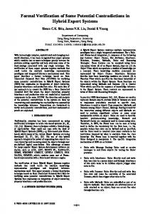
2 The LazyList Algorithm The LazyList algorithm implements a concurrent set supporting three operations: – add(k) adds k to the set and “succeeds” if k is not already in the set. – remove(k) removes k from the set and “succeeds” if k is in the set. – contains(k) “succeeds” if k is in the set. Each operation returns true if it succeeds; otherwise it “fails” and returns false. The algorithm uses a linked-list representation. In addition to key and next fields, each list node has a lock field, used to synchronise add and remove operations, and a marked field, used to logically delete the node’s key value (see Figure 1(a)). The list is maintained in ascending key order, and there are two sentinel nodes, Head and Tail, with keys −∞ and +∞ respectively. We assume that the list methods are invoked only with integer keys k (so that −∞ < k < +∞). As explained in more detail below, a successful add(k) operation inserts a new node containing k into the list, and a successful remove(k) operation logically removes k from the set by marking the node containing k (i.e., setting its marked field to true ), before cleaning up by removing the node from the list. Thus, at any point in time, the abstract set is exactly the set of values stored in the key fields of unmarked node in the list.

add(b)

private class Entry { int key; Entry next; boolean marked; lock lock; }

pred

curr

a

c

Head

Tail

b remove(b)

pred

curr

a

b

Head

Fig. 1. (a) Declaration of list node type,

Tail c

(b) Inserting and removing list nodes

The add(k) and remove(k) methods (see Figure 2) use a helper method locate(k), which sets curr to point to the first node with a key greater than or equal to k and pred to point to the node whose next field points to that node. The locate method optimistically searches the list without using locks, and then locks the nodes pointed to by curr and pred. If both nodes are unmarked (i.e., their marked fields are false ) and pred.next is equal to curr (these tests constitute three separate atomic actions), the add or remove operation can proceed; otherwise, the locks are released and the search is restarted. After locate returns, an add operation tests whether curr.key equals k. If not, then k is not in the list, so add creates a new node, setting its key field to k and its next field to point to curr (see Figure 1(b)). It then sets the next field of pred to point to this new node, releases the locks on curr and pred, and succeeds. If curr.key is equal to k, then k is already in the list, so the add operation fails. For a remove(k) operation, if curr.key equals k after locate returns, then remove removes the node at curr from the list and succeeds; otherwise, k is not in the list, so remove fails. A successful removal is done in two stages: first the key is logically removed from the set by setting the marked field of curr ; then it is physically removed by setting the next field of its predecessor (pred ) to its successor (curr.next ) (see Figure 1(b)). Separating the logical removal of the key from the set and the physical removal of the node from the list is crucial to the simplicity and efficiency of the algorithm: because nodes are not removed before they are marked, observing an unmarked node is sufficient to infer that its key is in the set. A contains(k) operation makes a single pass through the list, starting from Head, searching for a node with a key not less than k. If this node contains k and is not marked, contains succeeds; otherwise it fails. This operation requires no locks and is wait-free (i.e., it is guaranteed to complete within a finite number of its own steps, even if processes executing other operations are delayed or stop completely). Linearisation points A common way to prove that an algorithm is linearisable is to identify a particular step of each operation as the linearisation point of that operation. With some simple invariants showing there are no duplicate keys in the list, it is straightforward to assign linearisation points in this way for add and remove operations, and for successful contains operations. Things are not so simple for failed contains operations, however. If the node found by the loop at lines 2 and 3 contains a key greater than k, or it is marked, contains(k)

contains(k) : 1 curr := Head; 2 while curr.key < k do 3 curr := curr.next; 4 if curr.key = k and 5 ˜curr.marked then return true else return false locate(k) : while true do 1 pred := Head; 2 curr := pred.next; 3 while curr.key < k do 4 pred := curr; 5 curr := curr.next; 6 pred.lock(); 7 curr.lock(); 8 if ˜pred.marked and 9 ˜curr.marked and 10 pred.next = curr then 11 return pred, curr else 12 pred.unlock(); 13 curr.unlock()

add(k) : 1 pred, curr := locate(k); 2 if curr.key != k then 3 entry := new Entry(); 4 entry.key := k; 5 entry.next := curr; 6 pred.next := entry; 7 res := true else 8 res := false; 9 pred.unlock(); 10 curr.unlock(); return res remove(k) : 1 pred, curr := locate(k); 2 if curr.key = k then 3 curr.marked := true; 4 entry := curr.next; 5 pred.next := entry; 6 res := true else 7 res := false; 8 pred.unlock(); 9 curr.unlock(); return res

Fig. 2. Pseudo-code for lazy list algorithm

returns false. But there is no step of the contains operation at which k is guaranteed not to be in the set. In particular, when its key or marked field is checked, the node may have already been removed from the list, and another process may have added a new node with key k, so that k is in the abstract set at that time. Thus the simple approach of proving linearisability by defining a linearisation point for each operation at one of its steps does not work for this algorithm. The key to proving that LazyList is linearisable is to show that, for any failed contains(k) operation, k is absent from the set at some point during its execution. Our proof shows that if a contains(k) operation fails, then either k is absent from the set when it begins or that some successful remove(k) operation marks a node containing k during the execution of the contains(k) operation. Because there may be many contains(k) operations executing concurrently, it is sometimes necessary to linearise multiple failed contains operations after the same remove(k) operation. We found this interesting, because our previous proofs have not required this.

3 Verification To prove that LazyList is a linearisable implementation of a set supporting add, remove, and contains operations, we define two input/output automata (IOA) [9, 10]: a concrete automaton ConcAut, which models the behaviour of the LazyList algorithm, and a simple abstract automaton AbsAut, which specifies all correct behaviours of a linearisable set. We use simulation proof techniques [11] to prove that ConcAut implements AbsAut. 3.1

I/O automata and simulation proofs

We now informally describe the IOA model and simulation proofs. In our verification, we use a simplified version of IOAs, which is sufficient for this verification. See [9–11] for a more detailed and formal discussion. An IOA consists of a set of states and a set of actions. Each action has a precondition, which determines the set of states from which it can be executed, and an effect, which determines the next state after the action has been executed. The actions are divided into external actions, which define an interface to the automaton, and internal actions, which represent internal details. An automaton C implements an automaton A if for every execution of C, there exists an execution of A with the same external actions, which means that C cannot be distinguished from A by observing its external behaviour. One way to prove that C implements A is to consider an arbitrary execution of C and to inductively construct an execution of A with the same external actions in the following fashion: Start from the initial state in C’s execution, and then for each action in turn, choose a (possibly empty) sequence of actions for A to execute such that (i) the actions chosen constitute a valid execution of A, (ii) whenever C executes an internal action, the sequence of actions chosen for A has only internal actions, and (iii) whenever C executes an external action, the sequence of actions chosen for A contains that same action and no other external actions. In this way, we ensure that the constructed execution for A contains the same external actions as the execution of C. To describe this construction for an arbitrary execution, it is useful to define a forward simulation, which is a relation between states of C and states of A such that given a pair of states related by the simulation, and any action enabled in the state of C, there is a way to choose a sequence of actions for A that preserves this relation. For some algorithms and their specifications, however, there is no way to define such a forward simulation because for some action of C, the actions of A that we should choose depend on future outcomes. As we describe later, LazyList is one such algorithm. In such circumstances, a backward simulation can help. A backward simulation is like a forward simulation except that instead of starting from the initial state and working forwards to an arbitrary state of the automaton, we start at an arbitrary state and work backwards towards the initial state. For a backward simulation, we must be careful that while working backward, the abstract prestate that we end up at is reachable (going forward) from the initial state. Otherwise, we will not be able to construct an abstract execution that starts from the initial state. There is no similar proof obligation for forward simulations because every state resulting from executing an action from a reachable state is reachable by definition.

For this reason, and because thinking “backwards” seems less natural than thinking forwards, verifying backward simulations can be more challenging than verifying forward simulations. Furthermore, just as forward simulations are inadequate for some proofs, backward simulations are inadequate for others [11]. Therefore, when a backward simulation is necessary, it can be helpful to develop the proof in two stages by defining an “intermediate” automaton, and proving that the concrete automaton implements the intermediate automaton using a forward simulation and that the intermediate automaton implements the abstract one using a backward simulation. We have taken this approach for this verification, as we have used it successfully in previous verifications, e.g. [6]. 3.2

The abstract and concrete automata

We now describe informally the abstract and concrete IOAs that we use in this verification; more detailed descriptions of the way we use IOAs to model specifications and implementations can be found in [5–8]. The abstract automaton AbsAut models a set of processes operating on an abstract set, in which each process is either “idle”, in which case it can invoke any operation on the set, or is in the midst of executing an operation. There are four actions in AbsAut for the add method (see Figure 3). The addInv(k, p) action models invocation of the add method by process p with key k, and the addResp(b, p) action models this method returning boolean value b to process p. Between the invocation and the response, the automaton requires exactly one “do ” action, either a doAddT (p) or a doAddF (p) action. The precondition of the doAddT action requires that k is not in the abstract set, and its effect adds k to the set, and the doAddF action requires that k is in the set, and its effect does not modify the set. Each of the remove and contains methods is similarly modelled with four actions.

Action Precondition add(k, p) a‘pc(p) = idle doAddT(k, p) pcDoAdd(k) AND NOT member(k, a‘keys) doAddF(k, p) pcDoAdd(k) AND member(k, a‘keys) addResp(r, p) pcAddResp(r)

Effect a‘pc(p) := pcDoAdd(k) a‘pc(p) := pcAddResp(true) a‘pc(p) := pcAddResp(false) a‘pc(p) := idle

Fig. 3. AbsAut actions for the add method

Per-process program counter variables constraint the order in which actions can be performed, ensuring that each operation consists of an invocation action, a do action, and a response action. These variables also connect the return value of the response action to the do action. For example, the doAddT (p) action sets process p’s program counter to pcAddResp(true, p). Thus each operation is guaranteed to return a value consistent with applying the operation atomically at the point at which the do action

is executed. Because each operation “takes effect” atomically at the execution of its internal do action, all executions of AbsAut are behaviours of a linearisable set. Thus, proving that ConcAut implements AbsAut proves that LazyList is a linearisable set implementation. The concrete automaton ConcAut models a set of processes operating on a set implemented by the LazyList algorithm. It has the same external actions as AbsAut, but rather than modelling the application of the entire operation as a single atomic action, ConcAut has an internal action for each step of the algorithm corresponding to a labelled step in the pseudocode shown in Figure 2. In fact, conditional steps in the algorithm have two associated actions, one for each outcome of the step. For example, the precondition of the cont2T (p) action (which models an execution by process p of line 2 of the contains method when the test succeeds) requires that p’s program counter is pcCont2 and curr.keyp < kp , and its effect sets p’s program counter to pcCont3. 3.3

An intermediate automaton

As mentioned earlier, we cannot prove that ConcAut implements AbsAut using a forward simulation proof. The reason is that, to do so, we must identify a point at which each operation “takes effect” and choose the corresponding do action in AbsAut at that point. However, as explained in Section 2, a failed contains operation may not take effect at the point where it determines that it has failed: the point at which the sought-after key is absent from the set may be earlier. A correct forward simulation proof would have to choose the doContF action at a point where the key is absent from the set. However, at that point, it is still possible that the contains operation will return true, so choosing doContF would make it impossible to complete the proof because when ConcAut executes the external contResp(true) action, the precondition for this action would not hold in the AbsAut state (recall that we are required to choose the same action for AbsAut when the ConcAut action is external). The intermediate automaton IntAut must eliminate the need to “know the future” in order to choose appropriate actions in proving that ConcAut implements IntAut using a forward simulation. However, because backward simulations are more difficult than forward ones, we prefer to keep the intermediate automaton as close as possible to the abstract one. We achieved this by modifying AbsAut slightly so that the contains operation can decide to return false if the key it is seeking was absent from the set at some time since its invocation (though it is still permitted to return true if it finds its key in the set). We now explain how we achieved this. The state of IntAut is the same as that of AbsAut, except that we augment each process p with a boolean flag seen outp . When process p is executing a contains(k) operation, seen outp indicates whether k has been observed to be absent from the set since the invocation of the operation. The transitions of IntAut are the same as those of AbsAut, except that: – The contInv(p, k) action sets seen outp to false if k is in the abstract set, and to true otherwise. – The doRemT(q, k) action, having performed its usual action of removing k from the set, then sets seen outp for every process p that is executing contains(k).

– The precondition of the doContF(k, p) action is modified to require seen outp to be true instead of k being absent from the set. Thus the doContF(p) action is enabled if k was not in the set when contains(k) was invoked, or if it was removed later by some other process q performing doRemT(q, k). Therefore, in this automaton, a contains(k) operation can decide to return false even when k is in the set, provided k was absent from the set sometime during the operation. This is what we need in order to allow a forward simulation from ConcAut to IntAut. 3.4

The backward simulation

Because IntAut is so close to AbsAut, the backward simulation is relatively straightforward. Our simulation relation requires that the sets of keys in IntAut and AbsAut are identical, and that each process p in AbsAut stays “in step” with process p in IntAut, with one exception. In AbsAut, p may have already executed doContF, indicating that it will subsequently return false, whereas in IntAut, p has not yet decided to return false. This is allowed only if seen outp is true, indicating that either k is absent from the abstract set at the invocation contInv(k, p), or is present at the invocation but is subsequently removed before doContF is performed. The backward simulation relation has two components, one relating data and one relating program counters of processes. The PVS definition of our backward simulation relation between IntAut state i and AbsAut state a is shown below. bsr(i, a): bool = i‘keys = a‘keys AND FORALL p: (i‘pc(p) = a‘pc(p) OR (i‘pc(p) = pcDoCont AND a‘pc(p) = pcContResp(false) AND i‘seen_out(p)))

In the backward simulation, for each IntAut action, we choose the same action for AbsAut, with the following exceptions. First, for a doRemT(k, p) action in IntAut (which successfully removes k from the abstract set), we choose a sequence of AbsAut actions consisting of the same doRemT(k, p) action, followed by one doContF(k, p) action for each process p that is executing a contains(k) operation that is enabled to return false in the post state of AbsAut. Second, because we choose the doContF AbsAut action for a contains(k) operation that returns false in IntAut either at that operation’s invocation or in the sequence immediately after a doRemT action that removes k, doContF actions in IntAut are ignored (i.e., we choose not to execute any action in AbsAut for a doContF in IntAut). This corresponds to the intuition that, by the time IntAut decides to return false, the value it is seeking may actually be in the abstract set: it is at the point at which seen out is set to true that we know the value is absent, and therefore that is where we choose the doContF action for AbsAut. 3.5

The forward simulation

When defining the relationship between the states of IntAut and ConcAut, one option is to represent the relationship directly in the simulation relation. However, because

in this case the relationship is quite complex, we chose instead to reflect the state of IntAut within ConcAut via the introduction of two auxiliary variables, aux keys and aux seen out. Then, rather than constructing the simulation relation to directly relate the ConcAut state and the IntAut state, we capture this relation as invariants of ConcAut, and simply require that the auxiliary variables equal their counterparts in IntAut. This approach has the benefit of making it easier to check properties we intend to test with a model checker. ConcAut is augmented with the auxiliary variables in a straightforward manner: aux keys is updated when a node is inserted into the list at line 6 of the add method, or is marked for deletion at line 3 of the remove method; and aux seen outp is updated when the contains method is invoked by process p, or when another process executes line 3 of the remove method to remove the same value p is seeking. With the addition of the auxiliary variables, the simulation relation is quite simple. Like the backward simulation relation, it has two components, one relating data and one relating program counters of processes. The first component simply requires that the ConcAut auxiliary variables equal their respective counterparts in IntAut. The second component is more complicated than in the backward simulation relation, because we must relate each program counter of ConcAut to a program counter value in IntAut. The proof is also quite straightforward: almost all of the proofs for the forward simulation were dispatched automatically via the use of PVS strategies. The only proofs that required user interaction were those to show that whenever we choose a do action for IntAut or a given ConcAut action, that action’s precondition holds in IntAut. These proofs required the introduction of high-level invariants of the concrete automaton— one for each action corresponding to a do action in the intermediate automaton—that show that at the point that we choose these actions in the simulation, their preconditions hold in IntAut. For one interesting example, we must show that when we choose doContF(k, p) as the action for IntAut, seen outp is true. More specifically, we show that aux seen outp is true in the ConcAut state, and then use the simulation relation’s requirement that aux seen out and seen out are equal to infer that the IntAut action is enabled. Proving these invariants requires a number of other invariants and lemmas. Stating and proving these properties accounts for the bulk of the work in this proof. 3.6

Invariants

We do not have space to describe all of the invariants and properties we proved. Instead we choose a handful of interesting properties to discuss. The interested reader may examine the proofs in detail by consulting our proof scripts, which are available at http://www.mcs.vuw.ac.nz/reasearch/SunVUW/. The aux keys accurate invariant states that aux keys is exactly the set of keys for which there is a live node. (A live node is one that has been inserted into the list, and has not yet had its marked bit set.) This property is mostly straightforward because a key is inserted into aux keys each time a new node containing that key is inserted into the list (thus becoming live), and removed from aux keys each time a node containing the key is marked as deleted (thus ceasing to be live). The hardest part of this proof is showing that marking a node with a certain key value ensures that no live node with that key value

exists. This is achieved using several additional invariants: live nodes in list says that all live nodes are reachable from Head ; one from other says that if two different nodes are both reachable from Head then one of them is reachable from the other; and later nodes greater and public says that if one node is reachable from another, then it has a higher key. Together these three properties imply that there is at most one live node for a given key value at any time, and therefore marking one falsifies the existence of any such node, as required. A contains(k) operation that returns true finds an unmarked node containing k. Because the key field of a node does not change after it is initialised, if a contains(k) operation finds a node containing k and then observes that the node is not marked, it follows from aux keys accurate that k is in the abstract set when the node is observed to be unmarked. Thus, when we choose the doContT action for IntAut given a cont5T action in ConcAut, the precondition for doContT holds. A contains(k) operation that returns false is more interesting. When such an operation is invoked by a process p, if k is not in the abstract set, then by aux keys accurate there is no live node containing k, so the contInv(k, p) action sets seen outp to true. Therefore if the algorithm decides to return false, we are justified in choosing the doContF action for IntAut because its precondition holds. Otherwise, there is a live node containing k when the contInv(k, p) action is executed, and this is still true when the cont1 action reads Head unless the node has been marked, in which case seen outp (and aux seen outp ) are set to true, again justifying a subsequent execution of doContF in IntAut. Otherwise, after cont1 reads Head into currp , the live node is reachable from the node indicated by currp variable. As explained below, this remains true as p walks down the list towards the live node unless the live node is removed, setting seen outp to true. Thus, unless k is not in the set when contains(k) is invoked, or is removed before p reaches it, the contains(k) method returns true. The above reasoning is captured in part by the cont val still in invariant, which states that as p executes the loop at lines 2 and 3 of the contains(k) method, either aux seen outp is true, or there is a path from currp to a live node containing k. The latter property is captured by leadsfrom(currp , n), which states that there is a nonzero-length path from currp to n. leadsfrom is defined using leadsfromsteps as follows to allow us to prove to PVS that inductive proofs over it are finite. leadsfromsteps(c, n, m, w): INDUCTIVE bool = n /= Tail AND ((w=1 AND c‘nextf(n) = m) OR (w>1 AND c‘nextf(n) /= m AND leadsfromsteps(c,c‘nextf(n),m,w-1))) leadsfrom(c, n, m): bool = EXISTS w: leadsfromsteps(c, n, m, w)

A challenging part of the proof is proving that leadsfrom(m, n) is falsified only if node n is marked, and therefore cont val still in is not falsified by leadsfrom(currp , n) becoming false. The intuition for this property is clear: changes outside the path between m and n have no effect, and inserting or removing a node from the list between m and n preserves the leadsfrom(m, n) property. Thus, only removing a link to n can falsify leadsfrom(m, n), and it is easy to prove that this occurs only if n is marked. While the intuition for this property is straightforward, the

proof is somewhat involved because it requires various inductions over the leadsfrom property to capture the effects of inserting and removing nodes in the middle of the list. A key invariant that is used in many of the proofs, for example, capturing the effect of adding or removing a node, is the locate works invariant, which captures the properties that are guaranteed by the locate method because it locks the nodes and then validates the desired properties before returning to add or remove. Specifically, locate works tells us that when we return from a call to locate, we have locks on adjacent live nodes such that the key of the first node is smaller than our key, and the key of the second is greater or equal. Because we know (from live nodes in list and later nodes greater and public) that live nodes are in ascending order in the list, we can determine by examining the key of the curr node whether the value in question is in the abstract set or not. The locate works invariant also ensures, for example, that when rem5 sets the next field of its pred node to the value previously read from the next field of its curr node, the next field of the pred node still points to the curr node, thus ensuring that the intended node is the one removed. Another invariant entry unchanged in rem ensures that the value written to the next field of the pred node is still the next field of the curr node, showing that exactly one node (the curr node) is removed.

4 Experience with PVS We used PVS [4] to verify all the proofs discussed in this paper. As we are not experts in the use of PVS, and we had no special support, our experience may be relevant both to others considering using PVS to verify similar proofs, and as a comparison to others’ experience with different formal tools. In addition to our work with PVS, we collaborated with David Friggens and Ray Nickson, who developed models for this algorithm for use in the model checkers Spin and SAL [12, 13]. As well as model checking the entire algorithm for small numbers of threads and small bounds on the queue size, which gave us some confidence that our proof attempt would eventually be successful, they used these models to test some of the putative invariants we used in our proofs before we actually proved them. In approaching this verification, we worked mostly “top-down”, starting with the simulation proofs and then proceeding with the invariants. We did not develop the basic proof using PVS; rather, we figured out the top-level invariants informally, and prepared a fairly detailed proof sketch of these invariants, and some of their supporting lemmas and invariants, before formalizing them in PVS. We did not, however, work out all the low-level lemmas and invariants that we knew would be helpful for the proofs, leaving many of them to be stated and proved as necessary. As mentioned earlier, introducing auxiliary variables in the concrete automaton pushed the bulk of the work for this proof into the verification of invariants. The complete verification contained 171 PVS proofs: 27 typecheck constraints, 29 lemmas for the simulation proofs, and 115 invariants and supporting lemmas. Pushing most of the work into the invariants reduced the state that had to be managed within a PVS proof, because invariants are about a single automaton, while simulations are relations between two automata. Also, unlike simulation relations, invariants are straightforward to

check using model checkers, so this reduced the gap between our work and that of our colleagues working with Spin and SAL. PVS includes support for proof management, tracking which proofs have been done, and marking lemmas as proven but “incomplete” if they depend on earlier lemmas that have not yet been proved completely. This support helped us to work independently on different lemmas, which was especially helpful as the authors were spread over three countries. However, PVS manages changes at the file level—changes in the file invalidate all proofs for lemmas in that file—so we often had to rerun proofs that were unchanged. Finer-grained dependency tracking would have saved us considerable time. PVS supports the creation of user-defined rules, called strategies, by combining built-in rules. These strategies can be saved and used in other proofs (or several times in a single proof). We used strategies extensively, for example, to set up the beginning of invariant proofs, which almost always begin assuming the invariant holds on an arbitrary reachable state and setting up as a goal that it holds after executing any action; to extract parts of the precondition or effect of an action; and to handle the many “trivial” cases in the forward simulation proof for concrete actions that did not correspond to any action in the intermediate automaton. As useful as strategies are, we found that in many cases it was better to define a lemma that captured a desired property than to design a strategy to prove it. There are two advantages: First, PVS doesn’t have to do the proof each time—it just uses the lemma. Second, often the way you state a property makes a significant difference in how you are able to use it. With a lemma, you can easily control how a property is stated. Another disadvantage of strategies is that they are maintained in a single file, so defining new strategies invalidates all proofs, even those for lemmas in different files. One challenge in this verification was making proofs that PVS could check quickly. In particular, in an invariant proof, we typically show that the property is preserved by every action. Usually, only one or a few actions affect any of the variables mentioned by the property, and only those actions need to be considered; the rest obviously preserve the property. However, PVS must check all of those actions, and even a couple of seconds for each action turns into minutes for 52 actions. Thus, we stated and proved several “does not modify” lemmas, one for each variable, stating which actions actually modified that variable, and we used those lemmas extensively to avoid having PVS consider each of the other actions separately. We also found it helpful to define functions to describe things that we wanted to refer to frequently, and especially that we might want to use in a strategy. For example, in the forward simulation proof, we defined the action corr function to return, for any transition of the concrete automaton, the corresponding sequence of actions of the intermediate automaton. We also defined pcin and pcout to return, for each action, the program counters corresponding to the prestate and poststate respectively.

5 Concluding Remarks We have developed the first complete and formal correctness proof for the LazyList algorithm of Heller et al. [1]. We model the algorithm and specification as I/O Automata

in the PVS language, and proved that the algorithm implements the specification using simulation proofs developed in and checked by the PVS system. As in previous proofs we have done ([5–8]), we found that the outcome of an operation cannot always be determined before it takes effect. Our proof uses a combination of backward and forward simulations to deal with this problem. An interesting aspect of the proof, which we have not encountered in our previous proofs, is the need for multiple operations to be linearised after an action of a different operation. In a related manual verification effort, Vafeiadis et al. [14] consider a version of the LazyList algorithm that is augmented by adding auxiliary variables and actions that perform the abstract operation on an auxiliary set at the linearisation point of each operation, and use the Rely-Guarantee proof method [15, 16], to show that the implementation and the abstract set behave the same way in every execution of this augmented algorithm. Because it is impossible to correctly linearise a failed contains operation without knowledge of the future, this approach cannot be used to prove the linearisability of failed contains operations. Therefore, [14] only considers this case informally. Both our proof and our colleagues’ model checking work confirmed our doubts about some of the claims made about the linearisation points of failed contains operations in an early draft of [14]. Our completely machine-checked proof for the LazyList algorithm significantly increases confidence in the correctness of the algorithm. We have made out proof scripts available so that others may benefit from our experience (see http://www.mcs.vuw.ac.nz/reasearch/SunVUW/). We will also test our hypothesis that substantial parts of our proof can be reused to prove correct several optimised versions of LazyList. In the longer term, we plan to continue refining our proof methodology to make it easier and more efficient to develop fully machine checked proofs for concurrent algorithms. Acknowledgements: We are grateful to David Friggens and Ray Nickson for useful conversations and for model checking various proposed properties.

References 1. Heller, S., Herlihy, M., Luchangco, V., Moir, M., Scherer, W., Shavit, N.: A lazy concurrent list-based set algorithm. In: 9th International Conference on Principles of Distributed Systems (OPODIS). (2005) 2. Herlihy, M.P., Wing, J.M.: Linearizability: a correctness condition for concurrent objects. TOPLAS 12(3) (1990) 463 – 492 3. : (The PVS Specification and Verification System) 4. Crow, J., Owre, S., Rushby, J., Shankar, N., Srivas, M.: A tutorial introduction to PVS. In: Workshop on Industrial-Strength Formal Specification Techniques, Boca Raton, Florida (1995) 5. Doherty, S.: Modelling and verifying non-blocking algorithms that use dynamically allocated memory. Master’s thesis, School of Mathematical and Computing Sciences, Victoria University of Wellington (2003) 6. Doherty, S., Groves, L., Luchangco, V., Moir, M.: Formal verification of a practical lockfree queue algorithm. In de Frutos-Escrig, D., N´un˜ ez, M., eds.: Formal Techniques for Networked and Distributed Systems — FORTE 2004, 24th IFIP WG 6.1 International Conference, Madrid Spain, September 27-30, 2004, Proceedings. Volume 3235 of Lecture Notes in Computer Science., Springer (2004) 97–114

7. Colvin, R., Doherty, S., Groves, L.: Verifying concurrent data structures by simulation. In Boiten, E., Derrick, J., eds.: Proc. Refinement Workshop 2005 (REFINE 2005). Volume 137(2) of Electronic Notes in Theoretical Computer Science., Guildford, UK, Elsevier (2005) 8. Colvin, R., Groves, L.: Formal verification of an array-based nonblocking queue. In: ICECCS 2005: Proceedings of the 10th IEEE International Conference on Engineering of Complex Computer Systems, Shanghai, Chin (2005) 507–516 9. Lynch, N., Tuttle, M.: An Introduction to Input/Output automata. CWI-Quarterly 2(3) (1989) 219–246 10. Lynch, N.A.: Distributed Algorithms. Morgan Kaufmann (1996) 11. Lynch, N.A., Vaandrager, F.W.: Forward and backward simulations – part I: untimed systems. Information and Computation 121(2) (1995) 214 – 233 12. Holzmann, G.J.: The model checker SPIN. IEEE Trans. Softw. Eng. 23(5) (1997) 279–295 13. de Moura, L., Owre, S., Rueß, H., Rushby, J., Shankar, N., Sorea, M., Tiwari, A.: SAL 2. In Alur, R., Peled, D., eds.: Computer-Aided Verification, CAV 2004. Volume 3114 of Lecture Notes in Computer Science., Boston, MA, Springer-Verlag (2004) 496–500 14. Vafeiadis, V., Herlihy, M., Hoare, T., Shapiro, M.: Proving correctness of highly-concurrent linearisable objects. In: Principles and Practice of Parallel Programming (PPoPP), New York, USA (2006) Preliminary version: INRIA RR-5716 http://www.inria.fr/rrrt/rr-5716.html. 15. Jones, C.B.: Specification and design of (parallel) programs. In: 9th IFIP World Computer Congress (Information Processing 83). Volume 9 of FIP Congress Series., IFIP, NorthHolland (1983) 321–332 16. Xu, Q., de Roever, W.P., He, J.: The rely-guarantee method for verifying shared variable concurrent programs. Formal Aspects of Computing 9(2) (1997) 149–174