by translating the UML web service architecture description into a ... web design errors in an earlier stage, which are critical for web systems. Software ..... tocol RequestDataPacket, object A first sends object B a message ...... From our previous work [10], we know the generation of Petri nets ... Fundamentals of Algebraic.
Formalizing and Validating UML Architecture Description of Web Systems Yujian Fu, Zhijiang Dong, Xudong He Florida International University Miami, FL, 33199 {yfu002,zdong01,hex}@cis.fiu.edu
ABSTRACT Web systems are self-descriptive software components which can automatically be discovered and engaged, together with other web components, to complete tasks over the Internet. Unified Modeling Language (UML), a widely accepted object-oriented system modeling and design language, and adapted for software architecture descriptions for several years, has been used for the web system description recently. However, it is hard to detect the system problems, such as correctness, consistency etc., of the integration of Web services without a formal semantics of web services architecture. In this paper, we proposed an approach to solving this issue by translating the UML web service architecture description into a formal modeling language – SO-SAM, and verify the correctness of the web system design using model checking techniques. We presented this approach through an imaging processing scenario in the distributed web application.
Categories and Subject Descriptors D.2 [Software]: Software Engineering; D.2.4 [Software Engineering]: Software/Program Verification—formal methods, validation; D.2.11 [Software Engineering]: Software Architecture— Languages
General Terms UML architecture description, Verification
Keywords Software architecture model, verification and validation, Petri nets, Temporal logic
1.
INTRODUCTION
Web systems are self-descriptive software components which can automatically be discovered and engaged, together with other web components, to complete tasks over the Internet. The importance of web system architecture descriptions has been widely recognized in recently year. One of the main perceived benefits of a web system architecture description is that such a description facilitates system property analysis and thus can detect and prevent web design errors in an earlier stage, which are critical for web systems. Software architecture description and modeling of a web system plays a key role in providing the high level perspective, triggering the right refinement to the implementation, controlling the Copyright is held by the author/owner(s). ICWE’06 Workshops, July 10-14, 2006, Palo Alto, California, USA. ACM 1-59593-435-9/06/07.
quality of services of products and offering large and general system properties. While several established and emerging standards bodies (e.g., [6, 5, 3, 1, 2] etc.) are rapidly laying out the foundations that the industry will be built upon, there are many research challenges behind web system architecture description languages that are less well-defined and understood [25] for the large number of web service application design and development. On the other hand, Unified Modeling Language (UML), a widely accepted object-oriented system modeling and design language, has been adapted for software architecture descriptions in recent years. Several research groups have used UML extension to describe the web system’s architecture ([7, 21]). However, it is hard to detect the system problems, such as correctness, consistency [22] etc., of the integration of Web services without a formal semantics of web services architecture. Currently, although a software architecture description using UML extension contains multiple viewpoints such as those proposed in the SEI model [30], the ANSI/IEEE P1471 standard, and the Siemens [23]. The component and connector (C&C) viewpoint [32], which addresses the dynamic system behavioral aspect, is essential and necessary for system property analysis. To bridge the gap between web system architecture research and practice, several researchers explored the ideas of integrating architecture description languages (ADLs) and UML [8, 11, 12, 28]. Most of these integration approaches attempted to describe elements of ADLs in terms of UML such that software architectures described in ADLs can be easily translated to extensions of UML. There are several problems of the above approach that hinder their adoption. First, there are multiple ways to describe ADLs in terms of UML [18], each of which has advantages and disadvantages; thus the decision on which extension of UML to use is not unique. Second, modifications on UML models are difficult to be reflected in the original ADL models since the reverse mapping is in general impossible. Finally, the software developers are required to learn and use specific ADL to model software architecture and use the specific extension of UML, which is exactly the major cause of preventing the wide use of ADLs. Currently, there is less work involved to apply these methodologies to the web systems. In this paper, we present an approach opposite to the one mentioned above and apply our approach to the web applications, i.e. we translate a UML architecture description into a formal architecture model for formal analysis. Using this approach, we can combine the potential benefits of UML’s easy comprehensibility and applicability with a formal ADL’s analyzability. Moreover, this approach is used to formally analyze the integration of web services. The formal architecture model used in this research is named SOSAM, an extended version of SAM [19], which is based on Petri nets and temporal logic; and supports the analysis of a variety of
functional and non-functional properties [20]. Finally, we validate this approach by using model checking techniques. The remainder of this paper is organized as follows. In section 2, we review SO-SAM with predicate transition nets and temporal logic for high-level design. After that, we presented our approach in section 3 and the validation of the approach is demonstrated in section 4. Finally, we draw conclusions and describe future work in section 5.
2.
PRELIMINARIES
2.1
Overview of SO-SAM
SO-SAM [16] is an extended version of SAM [33] with the web service oriented features. SO-SAM [16] is a general formal framework for specifying and analyzing service oriented architecture with two formalisms – Petri Net model and temporal logic, which is inherited from SAM. In addition, SO-SAM extended the net inscriptions with servicesorts and net structure with initial and f inal ports that carry service triggering information. Furthermore, SO-SAM restricted SAM connector without hierarchical architecture. Finally, SO-SAM component is described by WSDL or XML. Also, the message in ports is defined by XML message. For the more information, please refer to [16]. In this paper, we choose algebraic high level nets [15] and linear time first order temporal logic as the underlying complementary formalisms of SAM. Thus, next we simply introduce the algebraic high level nets used in our approach.
2.1.1
Algebraic High-Level Nets
An algebraic high-level net integrates Petri net with inscription of an algebraic specification defining the data types and operations. Instead of specifying a single system model, an algebraic Petri net represents a class of models that often differ only in a few parameters. Such a compact parameterized description is unavoidable for modular specification and economic verification of net models in the dependable system design. Generally speaking, an algebraic high-level (AHL) nets N = (S PEC, A, X, P, T, W + , W − , cond, type) consists of following parts: • An algebraic specification S PEC = (S , OP, E), where S IG = (S , OP) is a signature with set of sorts and operations, and E is a set of equations over S IG; • A is a S PEC algebra; • X is a family of S-sorted variables; • P is a set of places; • T is a set of transitions such that P ∩ T = ∅; • Two functions W + , W − assigning to each t ∈ T an element of the free commutative monoid 1 over the cartesian of P and terms of S PEC with variables in X. • cond is a function assigning to each t ∈ T a finite set of equations over signature S IG. • type is a function assigning to each place a sort in S .
2.1.2
Linear Temporal Logic
Temporal formulas [27] are built from elementary formulas using logical connectives ¬ and ∧ (and derived logical connective ∨, 1 A set M with an associative operation ∗ and an identity element for that operation is called a monoid. A commutative monoid is a monoid in which the operation is commutative. A commutative monoid is a free commutative monoid if every element of M can be written in one and only one way as a product (in the sense of ∗) of elements of subset P M.
⇒, and ⇔), universal quantifier ∀ (and derived existential quantifier ∃), and temporal operators always �, future ^, until U and next d. The semantics of temporal logic is defined on behaviors (infinite sequences of states). The behaviors are obtained from the execution sequences of petri nets where the last marking of a finite execution sequence is repeated infinitely many times at the end of execution sequence. For example, for an execution sequence M0 , ..., Mn , the following behavior σ =� M0 , ..., Mn , Mn , ... � is obtained, where Mi is a marking of the Petri net. Let σ =� M0 , M1 , ... � be the behavior, where each state Mi provides an interpretation for the variables mentioned in predicates. The semantics of a temporal formula p in behavior σ and position j is denoted by (σ, j) |= p. We define: • For a state formula p, (σ, j) |= p ⇔ M j |= p; • (σ, j) |= ¬p ⇔ (σ, j) 6|= p; • (σ, j) |= p ∨ q ⇔ (σ, j) |= p or (σ, j) |= q; • (σ, j) |= �p ⇔ (σ, i) |= p for all i ≥ j; • (σ, j) |= ^p ⇔ (σ, i) |= p for some i ≥ j; • (σ, j) |= pUq ⇔ ∃i ≥ j : (σ, i) |= q, and ∀ j ≤ k < i, (σ, k) |= p;
2.2
Component and Connector View
Component and connector view was one of the four views proposed in [23, 24], which is described as an extension of UML. The component and connector view describes architecture in terms of application domain elements. In this view, “the functionality of the system is mapped to architecture elements called components, with coordination and data exchange handled by elements called connectors.” [23] In the UML 2.0 [4], composite structure diagram is developed for the description of interacted entities. This part extends UML description to the composition of elements using the concepts like ports, components and connectors etc.. The method for these elements description is compatible with those Clements’ methods [30]. However, the structures are too complicated, implementation-oriented, and connector and port are not in a uniform. These notations are general notations, and not specific for architecture documentation. Therefore, we choose the notation in the work [30]. In the component and connector view, components, connectors, ports, roles and protocols are modelled as UML stereotyped classes. Each of them is represented by a special type of graphical symbol, as summarized in Fig. 1. A component communicates with another component of the same level only through a connector by connections, which connect relevant ports of components and roles of connectors that obey a compatible protocol. In addition to the connections between components and connectors, ports (roles, resp.) of a component (connector, resp.) can be bound to the ports (roles, resp.) of the enclosing component (connector, resp.). In order to present our approach we use an image processing example used in the distributed web application that was adapted from [23]. Image processing is responsible for framing raw data into images and feed to the web application for the image transferring. Fig. 2, 3, 4 from [23] show a concrete and complete component and connector view, which is the running example of this paper. Fig. 2(a) is a configuration of ImageProcessing component. Fig. 2(b) shows another aspect of the configuration. Both of them are UML class diagrams and model different aspects of the system. From these two figures, we can see the component ImageProcessing contains
Element/Relation
UML Notation
component
Class
connector
Class
role
Class
port
Class
protocol
Class
composition
Composition
binding
Association
connection
Association
Graphical Symbol
obeys
Association
obeys
obeys conjugate
Association
obeys conjugate
Figure 1: UML Extension for component and connector View
two components: Packetizer and ImagePipline, and one connector PacketPipe. The ports of component ImageProcessing, rawDataInput, acqControl, and framedOutput are bound to ports rawDataInput of component Packetizer, acqControl and framedOutput of component ImagePipeline respectively. Component Packetizer communicates with component ImagePipeline through connector PacketPipe. Component Packetizer and connector PacketPipe are connected by a connection between port PacketOut and role source, which obey (conjugate) protocol DataPacket. Component ImagePipeline and connector PacketPipe are connected by a connection between port PacketIn and role dest, which obey (conjugate) protocol RequestDataPacket. Being a conjugate means that the ordering of the messages is reversed so that incoming messages are now outgoing and vice versa. acqControl ImageProcessing
acqControl rawDataInput Packetizer rawDataInput
PacketOut
packetIn PacketPipe
source
framedOutput
ImagePipline
dest
by a stereotyped class, is defined as a set of incoming message types, a set of outgoing message types and the valid message exchange sequences. The valid message exchange sequence is represented by a sequence diagram. Fig. 3 shows the definition of RawData, DataPacket, and RequestDataPacket protocols. From Fig. 3(c), we can see protocol RequestDataPacket has one incoming message: packet(pd), and three outgoing messages: subscribe(c), desubscribe(c), and requestPacket(c) where c, pd are parameters of messages. In order to communicate with object B based on protocol RequestDataPacket, object A first sends object B a message subscribe(c) where c indicates the sender A. Then a message requestPacket is sent to B to request a packet. Later, object A may receive a packet pd from B. The symbol “*” in the figure indicates that the pair of message requestPacket and packet(pd) may occur many times. Finally, object A sends a message desubscribe(c) to B to stop requesting packet. The behavior of components/connectors may be described formally by UML statechart diagrams, for example the behavior of component Packetizer and connector PacketPipe in Fig. 4. Statechart diagrams describe the dynamic behaviors of objects of individual classes through a set of conditions, called states, a set of transitions that are triggered by event instances, and a set of actions that can be performed either in the states or during the firing of transitions. From Fig. 4(b), we can see the statechart diagram of connector PacketPipe contains two states: waiting and “assign packet to ready client” and seven transitions. When connector PacketPipe receives an event subscribe(c), it invokes its operation AddClient(c) although we do not know exactly the functionality of this operation. When the connector receives an event packet(pd), it saves the packet pd. And the response of connector PacketPipe to an event requestPacket(c) is up to the condition: the client c has read current packet or not. If yes, the connector treats it as a request for next packet; otherwise it sends current packet to client c through an event c.packet(pd). If all clients have read current packets, the connector updates its packet queue and enter state ”assign packet to ready client” in which the connector sends current packet to clients that has submitted their requests. If all requests are processed, the connector return to state waiting. As we can see from this figure, connectors and components mainly handle incoming messages of protocols they obey (conjugate).
framedOutput
(a) Component ImageProcessing
Packetizer
init packet
PacketPipe
�
�
�
�
�
��
��
��
��
�
�
�
�
�
ImagePipeline
idle
[packetFull]/ packet(pd)
[packetNotFull]
dataReady/ requestData
�
�
add data to packet
rawDataInput
connection
packetOut obeys
RawData
DataPacket
source
dest
obeys conjugate
PacketIn obeys
rawData(rd)
waiting
connection
obeys conjugate
RequestDataPacket
(a) Behavior of Component Packetizer subscribe(c) /AddClient(c)
(b) Protocols for Packetizer and PacketPipe
waiting packet(pd) /AppendQueue(pd)
Figure 2: Structural Aspect of Component and Connector View Fig. 2 alone is not enough to illustrate component and connector view since only components and connectors of the system and corresponding connections among them are demonstrated. Additional diagrams are needed to define protocols and functional behavior of components and connectors. A protocol, represented
desubscribe(c) /RemoveClient(c)
requestPacket(c) [packet not read] /c.packet(pd)
[IsClientReady(c)] /c.packet(pd)
[no client ready] assign packet to ready client [packet read by all] /UpdatePacket() requestPacket(c)[packet read] /SetClientReady(c)
(b) Behavior of Connector PacketPipe
Figure 4: Behavior of Elements
� �
� � �
�
� �
� �
�
��
�
�
RawData � �
� �
� �
� �
Packetizer � �
dataReady
incoming dataReady rawData(rd) outgoing
� �
�
� �
�
� �
rawData(rd)
� �
� �
�
� �
�
� �
ImagePipeline
RequestDataPacket
incoming
subscribe(c)
incoming
packet(pd)
requestData
� �
�
Packetizer
DataPacket
� �
packet(pd) � �
� �
� �
*requestPacket(c) � �
� �
� �
� �
outgoing subscribe(c) desubscribe(c) requestPacket(c)
outgoing
requestData
packet(pd)
(a) Protocol RawData
(b) Protocol DataPacket
*c.packet(pd) desubscribe(c)
(c) Protocol RequestDataPacket
Figure 3: Protocols in Component ImageProcessing
3.
TRANSFORMATION FROM COMPONENT & CONNECTOR VIEW TO SO-SAM
Component and connector (C&C) view [32] has been the main underlying design principle of most ADLs [29], which is also a major view type in several software architecture documentation models supporting multiple architecture views such as SEI [30] and Siemens [23]. C&C view is essential and necessary for system dependability analysis since it captures a system’s dynamic behavioral aspect. SO-SAM model and component and connector view share a set of common terms such as components, connectors, and ports. Therefore it is straightforward to map them to the counterparts in SO-SAM. However, due to the meaning difference and various formal methods to describe elements’ behavior, the concrete mapping procedure is not that easy. This section shows a method to construct a complete and executable SO-SAM model from a component and connector view. A component (connector, resp.) in component and connector view is mapped to a component (connector, resp.) in SO-SAM model. It is easy to understand from structural aspects. However, the behavior mapping is complex since different formal methods are used to model behavior. UML statechart diagrams are used to model behavior in component and connector view, contrasting with Petri net model in SO-SAM. Fortunately, our previous work [10] showed that it is possible to transform statechart diagrams to Petri net models. In UML statechart diagrams, method invocations and relationships between variables are implicit in the elements’ structure. For example, in Fig. 4(a), the conditions PacketNotFull and PacketFull, and relationship between variable rd and pd is not illustrated explicitly. However, such information has to be expressed explicitly in order to obtain a complete and executable Petri net. In order to bridge the gap, we utilize algebraic high level nets [15], a variant of high level Petri nets, to model behavior of elements. This method is possible because SO-SAM model does not specify a particular Petri net model as its formal foundation. We use algebraic specifications [13] to capture structures of elements obtained from UML statechart diagrams because algebraic specifications are abstract enough that no additional information about implementation detail is assumed, and they are also powerful enough to represent implied information about components or connectors. Although the work [10] is for SAM architecture model, we can still use it and adapt it to the SO-SAM model since they share the same net structure. The main differences exist in the service sorts in the net specification, initial and final ports in the net specification and net inscription. The following rule gives us a general idea to derive components or connectors in SO-SAM. RULE 1 (C OMPONENT AND C ONNECTOR ). A Component (connector, resp.) in component and connector view is mapped to a component (connector, resp.) in SO-SAM according to following
steps: Step 1 An algebraic specification, which specifies the abstract interface of the component (connector, resp.), is generated from a UML statechart diagram. The idea to construct algebraic specification is described later. Step 2 Construct a complete and executable algebraic high level net from the UML statechart diagram according to the approach in [10] and the generated algebraic specification. There is a special place in the generated algebraic high level nets that contains element information and provides necessary information for transitions. Step 3 A component (connector, resp.) with a UML statechart diagram in component and connector view is mapped to a component (connector, resp.) with an algebraic high level net in SO-SAM. While it is inherently impossible to prove the correctness of the transformation, we have carefully validated the completeness and consistency of our transformation rule. First, from structure point of view, concepts of components or connectors in component and connector view and SO-SAM are the same. Both of them support composition, binding with enclosing element, and they can have their own behavior and communication channels–ports or roles. Therefore, the main functionalities of components or connectors in component and connector view are presented in SO-SAM counterparts. Second, algebraic specification can be used to specify modular, more specific classes [14]. Therefore, the implied information of statechart diagrams, i.e. the operations and their properties can be correct and fully specified by algebraic specifications. Since functions of algebraic specifications only define what to be done, no additional implementation information not implied in statechart diagrams is introduced. Finally, our previous work [10] and others work [31] have shown that the behavior described by statechart diagrams can be fully captured by corresponding Petri nets. The idea to obtain algebraic specifications from UML statechart diagrams is as follows: For each element (component and connector), its algebraic specification defines a sort, called element sort, like packetizer for component Packetizer and packetpipe for connector PacketPipe. If a data type of parameters is not defined by a primitive algebraic specification, a new algebraic specification is imported. Such a imported algebraic specification generally defines only one sort, like Packet for component Packetizer. Each action of transitions in a UML statechart diagram is considered as a function such that: action name : element sort × parameters sort list → element sort. Here parameters sort list includes service sorts as well. For a guard condition of a transition, a function from element sort (with necessary parameter sorts) to boolean is added. For each variable that is defined in the element (i.e. the variable is not defined in the related events), a function like GetVariableT ypeName :
rawdata(rd)
t2 18
t2 12
t2 11
dataReady idle
t2 14 p.PacketNotFull()
init_packet
RECV
t2 13 t2 waiting 15
requestData rawdata(rd) SEND
pd
t2 16
t2 17
p.PacketFull() ^ =p.GetPacket()
p
p
add_data
p
p p’
packetizer
p’=p.AddRawData(rd)
(a) Petri net for Packetizer p’=p.AddClient(c) PacketPipe p
p’
p’=p.RemoveClient(c) p t2 22
p
t2 25 p.IsClientReady(c) ^ (p’,pd)=p.GetPacket()
p
t2 23
p t2 24 p.NoClientReady() c.packet(pd)
subscribe(c)
t2 21
desubscribe(c) waiting
RECV
packet(pd)
t2 26
RequestPacket(c)
p.PacketRead() t2 27
assign
c.packet(pd)
t2 28 p.ReadByAll() p
p p
SEND
RequestPacket(c)
p’=p.SetClientReady(c)
p.PacketNotRead()^ (p’,pd)=p.GetPacket() t2 29 p’=p.UpdatePacket()
PacketPipe
p
p’
p’=p.AppendPacket(pd)
(b) Petri net for PacketPipe
Figure 5: Behavior of Elements element sort → element sort × VariableT ype 2 is specified. The properties of these functions can be constructed as equations if they are implied in the UML statechart diagrams, like guards PacketNotFull and PacketFull cannot hold at the same time. From the above idea, we know that the algebraic specification for component Packetizer contains four functions, two of them correspond to guard conditions: .PacketNotFull(), .PacketFull() : packetizer → bool; and one is obtained from actions: .AddRawData( ) : packetizer × rawdata → packetizer, and one from undefined variable: .GetPacket() : packetizer → packetizer × packet. In these functions, “ ” is used to indicate a variable placeholder, bool is a sort defined in primitive algebraic specification Bool [13], and sorts rawdata and packet are defined in imported algebraic specifications Packet and RawData respectively, which are defined by users and normally only one sort (rawdata, packet resp.) is specified. With these algebra specifications, we can generate corresponding algebraic high level nets according to Rule 1. Fig. 5 shows the generated Petri nets from UML statechart diagrams in Fig. 4. Each generated Petri net has three special places: RECV containing messages from environment, SEND temporarily storing messages generated for its environment, and the place whose name is the same as its element’s name (here, Packetizer and PacketPipe resp.), holding the abstract structural information of the element. In additional to these three places, there is a corresponding place indicating current status for each state in statechart diagrams, for example, places idle,waiting, init packet and add data for the same name states. A special token in these places indicates if the corresponding state is active. Place RECV sends events from external environment to places that are interested in the event. In Fig. 5(a) place idle and waiting are interested in event dataReady and rawdata(rd) respectively. If state idle is active and an event dataReady is available,
2 transition t15 is fired. As a result, an event requestData is added to place SEND, and place waiting becomes active. State add data becomes active if state waiting is active and an event rawdata(rd) is available. At the same time, the token in place packetizer is changed to another one through operation .AddRawData( ) of algebraic specification Packetizer. Components and connectors in component and connector view are connected through a connection if they are enclosed directly by the same element and the corresponding ports and roles obey (conjugate) a compatible protocol. Therefore, the mapping from ports or roles in component and connector view to ports in SO-SAM is actually the mapping from relevant protocols describing behavior of ports or roles to ports of SO-SAM components/connectors. However, ports in SO-SAM models have their own characteristics. A port in SO-SAM model is a place that has either no incoming arcs or no outgoing arcs. In other words, the communication between ports is unidirectional. Therefore, a protocol in component and connector view, which consists of a set of incoming message types, a set of outgoing message types and the valid message exchange sequences, is mapped into a set of interface places (To avoid confusion, we use interface places to refer to ports in SO-SAM model). The type of tokens in an interface place is OID × OID × MES S AGE T Y PE, where OID is a set of unique identification number for each instance of the element, which specifies sender and receiver of a message, and MESSAGE TYPE is the set of message types of the protocol (Here we ignore the parameters of messages for brief). Rule 2 specifies how to map a port/role in component and connector view to interface places in SO-SAM. 2 This is actually the abbreviation of two functions: GetVariable : element sort → VariableT ypes and U pdateElement : element sort → element sort since these two functions are invoked sequently in our example.
RULE 2 (P ORTS AND ROLES ). A port (role, resp.) of a component (connector, resp.) in component and connector view is mapped to a set of interface places of the corresponding component (connector, resp.) specified by Rule 1: For each protocol that the port (role, resp.) obeys (conjugate), each kind of incoming messages is mapped to an incoming (outgoing, resp.) interface place of the component (connector, resp.) with the name of the message type; and each kind of outgoing messages is mapped to an outgoing (incoming resp.) interface place of the component (connector, resp.). Initial and final ports can not be obtained from the UML architecture description directly. We provided two possible solutions: • One is extending C&C view with new UML stereotypes initialPort and f inalPort. This would bring a direct transformation from C&C architecture to SO-SAM. The problem is this also bring more complexity into UML architecture description. • Another is manually adding the specification for these ports according to the system architecture description. For instance, we can say dataReady and RawData as initial port and frameOut as final port in our case. A port (role, resp.) of an element is actually –roughly speaking– a “channel” that forwards messages of specified types either from element itself to environment, or from environment to element. In Rule 2, a token represents an occurrence of an message of specified type, and the direction of a message is specified by the place containing the token – incoming or outgoing. Therefore, the mapping in Rule 2 conserves the main structural features of ports/roles and related protocols, and the reverse mapping exists, which ensures the correctness of the rule.
The behavior of a protocol, defined by UML sequence diagrams to demonstrate valid message exchange sequences, actually specifies possible sequences of relevant messages along time axle. A sequence of protocol messages illustrates their occurrence order, which can be specified by a set of temporal constraints, the basic predicates of which are the names of interface places obtained through Rule 2. For example, from Rule 2, we know port RawData of Packetizer is represented by two incoming places dataReady and rawData, and one outgoing place requestData. We use predicate dataReady(< sid, rid, mdataReady >) to describe if place dataReady contains a token representing an event dataReady that is sent to rid by sid. In order to construct temporal constraints, we consider two elements communicating with each other through a protocol, for example RawData. First we only consider a pair of adjacent events, for example DataReady and requestData. For this pair of events, it means if an event DataReady occurs, then an event requestData must occur some time later, which is described by a temporal formula: ∀ , �(dataReady() → ^ requestData()) (1) However, this temporal formula cannot reflect the situation implied in the sequence diagram of the protocol: no other events of the protocol can occur between events dataReady and requestData. In order to describe this implied property, we have a reasonable assumption at architecture level that the communication media is reliable, no message is lost and no need to resend a message. Therefore, another temporal formula is introduced to address this missing situation: ∀ , �(dataReady() → ¬(( ddataReady( )) ∨ requestData() ∨ rawData())U requestData()) (2) This temporal formula means if an event of dataReady occurs, no other events such as dataReady, requestData and rawData can occur before the first event of requestData. Predicate ddataReady(< sid, rid, md>) is used to guarantee that the temporal formula is satisfied at the time the event dataReady occurs. Therefore, given a sequence diagram of a protocol with n messages, we can obtain (n − 1) ∗ 2 temporal formulas. In addition to the consideration of one session of a protocol, we have to inspect the relationship of two adjacent sessions of the same protocol between two objects, i.e. one session can start only after the previous session ends. Such a relationship is specified by a temporal constraint: ∀ , �(rawData() → ¬(dataReady() ∨ requestData() ∨ ( drawData()))U dataReady()) (3) Although we think the above generated constraints are strong enough, there is still one more case we ignored: the first session of a protocol in a running system may starts with any messages but the first message. For example, a session of protocol RawData starts with message dataReady, and then obeys relevant part of the sequence diagram. We can see this session satisfies the above temporal formulas, but conflicts with the behavior of the protocol. Such a case can be avoided in three different ways, and the choice of them is up to users. One is to introduce a temporal predicate basetime that holds only at the time “zero”, and a new temporal formula: �(basetime → ¬(dataReady() ∨ requestData() ∨ rawData())U dataReady()) (4) The second method is to introduce a past time operator such as “eventually in the past”. The final way is to prove that system structure guarantees that such case cannot happen. Thus, from the above discussion, a sequence diagram for a protocol is mapped to a set of temporal constraints.
The following rule is used to construct a set of constraints for components or connectors according to the above discussion. RULE 3 (C ONSTRAINT ). For each protocol that a port (role, resp.) obeys (conjugate), a set of constraints, generated from the corresponding sequence diagram according to the above discussion, is added to the property specification of corresponding components (connectors, resp.) . When a constraint is added to a component (connector, resp.), sid or rid in tokens (the choice is up to the direction of corresponding message) is substituted by the actual identification number of the component (connector, resp.) since the component (connector, resp.) can only receive messages sent to itself. A sequence diagram of a protocol specifies possible message communication sequences. However, it is impossible to limit the firing sequences of transitions in Petri nets to meet specified occurrence sequences of tokens in places. Although we cannot specify the firing sequences of transitions, but we can prove that if each possible firing sequence meets the behavior of a protocol. From the above discussion, we can see the generated set of temporal formulas exactly realizes the behavior of a protocol – the message sequences. By adding these temporal formulas as property specifications to components/connectors obeying the protocol, inconsistencies between behavior of elements and protocols can be easily detected. Since the behavior mapping in Rule 1 is complete and consistent, we know the detected inconsistencies also exist in the original model, i.e. Rule 3 is complete and consistent. We may obtain a component (connector, resp.) with a behavioral model, and related ports and constraints according to Rules 1, 2 and 3 respectively. Next task is to get a complete component or connector, i.e. ports of a component or connector has to be integrated with its behavior model. Rule 4 is used to guide such a procedure, and Rule 5 establishes the connection between components and connectors. RULE 4 (I NTEGRATION ). The interface places, i.e. ports of a component (connector, resp.) in SO-SAM are integrated into its behavior model with the previous generated algebraic high level nets according to the following steps: Step 1 Each incoming interface place is connected to place RECV through a transition, firing of which transmits tokens in the incoming place that are sent to the instance of component or connector to place RECV unconditionally. Step 2 Each outgoing interface place is connected to place SEND through a transition, which forwards tokens of a special type in place SEND to the outgoing place. RULE 5 (C ONNECTION ). From Rules 2 and 4, if there is a connection between ports of a component and a role of a connector, then generated behavior models of the component and connector share a set of places that corresponds to the protocol they obey (conjugate). Therefore, to establish the connection between a component and a connector in SO-SAM, we merge these shared interface places because an incoming (outgoing, resp.) interface place in the component has an outgoing (incoming, resp.) counterpart in the connector such that they contain messages of the same type, and vice versa. In component and connector view, relationships between ports and behaviors are not specified explicitly. A port forwards incoming messages to the queue of the component/connector, which provide events for its behavior – the statechart diagram. The statechart
diagram sends messages to its environment through a port. In Rule 4, place SEND serves as output queue and place RECV is input queue. The forward action is represented by the firing of transitions connecting place SEND, RECV and other interface places. Therefore Rule 4 captures the communication between ports and the corresponding behaviors in component and connector view. Due to the space limitation, we cannot specify the transformation of binding and multiplicity. However, such transformations are similar and straightforward. Fig. 6 shows the final result of generated SO-SAM model from the running example. In order to give a concise description, algebraic specifications and internal parts of behavioral models are omitted. acqControl
ImageProcessing
t1 31 PacketPipe dataReady t1 rawData111 t 12 t1 13 requestData
2 dataReadyt19
RECV
t2 110 rawData t2 111
SEND
t2 29
acqControl packet
subscribe t2 210 packet RECV desubscribe t2 211 requestData SEND t2 t2 112 213 t2 212 requestPacket Packetizer
frameOut frameOut t1 32 ImagePipeline
Figure 6: ImageProcessing in SO-SAM
In Fig. 6, components, for example component Packetizer and component ImageProcessing are represented by solid rectangles, while connectors such as PacketPipe are represented by dashed rectangles. The Petri nets enclosed by rectangles are the behavior models of components or connectors. Semicircles on the edge of rectangles are places that represent ports derived from relevant protocols. An inside semicircle indicates an incoming place that only receives tokens from environment, while an outside semicircle indicates an outgoing place that only sends tokens to environment. For example, component Packetizer has two incoming places dataReady, rawData, and one outgoing place requestData. These three places are derived from protocol RawData according to Rule 2. Component Packetizer and connector PacketPipe is connected through Rule 5. The binding between components and its enclosing component is implemented as a transition between corresponding places, which only forwards tokens from one place to another according to types of places (i.e. incoming or outgoing). For ex1 ample, transition t11 forwards tokens in place dataReady of ImageProcessing to place dataReady of Packetizer, while transition 1 t13 forwards tokens in place requestData of Packetizer to place requestData of ImageProcessing. Finally, we give an execution path of component ImageProcessing. Let component Packetizer be in state idle, connector PacketPipe in state waiting, and place ImageProcessing.dataReady contains a token representing message dataReady. This initial condition can be represented by the initial marking (ImageProcessing.dataReady, Packetizer.idle, PacketPipe.waiting). Here we only list related places (not including places such as packetizer and PacketPipe) that contain tokens, and ignore concrete token values that can be derived from context. We also assume that a packet consists of only one raw data, i.e. operation PacketFull() will be true if AddRawData() is invoked once. Table 1 shows the execution of communication based on protocols RawData and DataPacket. This example demonstrates the application of our method.
4.
VALIDATION OF THE APPROACH
The SO-SAM model allows formal validation of a service net against system constraints and property specified on its abstraction
represented by a component or connector. Here, validation means that the developer can animate the specification by providing initial markings and checking if the responses meet the expected results. Validation of SO-SAM is based on the precise syntax and semantics of Petri net formal language and temporal logic. The validation will cover the topology and dynamic behavior of the Petri net as well as temporal logic formulae. Here we simply introduce how to translate SO-SAM model to the Maude [9] language. For the details, please refer to the work [17].
4.1
Translation from SO-SAM to Maude
Step 1. Translation to the functional module: generate the sorts operators used in the functional modules for the model signatures. This step translates each place, sorts, markings in a Petri net into the corresponding part in Maude’s functional module. Step 2. Translation to the system modules: there are three types of system modules, one is for the model signature that corresponds to the architecture structure and dynamic behavior of the model, one is for the mapping to the predicates, and one is for the model checking, which includes the property specification. 1. Each basic component and connector are defined as a system module (SysID) with the declaration of variables and necessary rules and operators. Each composition is specified as a system module that including its sub-components and connector that are predefined as a module. All guard conditions in a transition are a (un)conditional rule. 2. Each place is mapped to an operator in the predicate system module (SysID-PREDS). The connection between operators and predicate is established by an equation. 3. Model checking module (SysID-CHECK) is mainly for the initial marking and property specification. In our translation, system signature such as sorts and operators are declared in the functional module. This translates the places/ports, sorts into algebra in Maude that will be used in the system modules. The dynamic semantics of Petri net can be mapped to the rewriting rules used in Maude. Computationally, the meaning of rewriting rules is to specify local concurrent transitions that can take place in a system if the pattern in the rule’s lefthand side matches a fragment of the system state and the rule’s condition is satisfied. In that case, the transition specified by the rule can take place, and the matched fragment of the state is transformed into the corresponding instance of the righthand side. Thus we can see an amazing match between semantics of Petri net and rewriting logic. These are theoretic aspect of the above translation algorithm.
4.2
Results
The basic requirements for the image processing in the distributed web applications are correctness, robustness and reliability. We use model checker of Maude [9] to validate the SO-SAM model obtained from UML architecture description against system properties. After studying models and the errors discovered during the model validation, two main property categories have been selected: 1. Structural properties: this kind of properties is closely related to the topology of the model. These properties can be directly verified on the SO-SAM model without animating the transactions. These properties are necessary conditions that ensure the feasibility of the state transitions. If one of them is not fulfilled, we can assert firmly that the communication between ports in UML description cannot happen.
Step 1 2 3 4 5 6 7 8 9 10 11 12 13 14 15 16 17 18
Marking of Component ImageProcessing idle, ImageProcessing.dataReady, PacketPipe.waiting idle, Packetizer.dataReady, PacketPipe.waiting idle, Packetizer.RECV, PacketPipe.waiting idle, PacketPipe.waiting Packetizer.waiting, Packetize.SEND, PacketPipe.waiting Packetizer.waiting, Packetizer.requestData, PacketPipe.waiting Packetizer.waiting, ImageProcessing.requestData, PacketPipe.waiting Packetizer.waiting, PacketPipe.waiting Packetizer.waiting, ImageProcessing.rawData, PacketPipe.waiting Packetizer.waiting, Packetizer.rawData, PacketPipe.waiting Packetizer.waiting, Packetizer.RECV, PacketPipe.waiting Packetizer.waiting, PacketPipe.waiting Packetizer.add data, PacketPipe.waiting Packetizer.initial packet, Packetizer.SEND, PacketPipe.waiting, Packetizer.idle, Packetizer.SEND, Packetpipe.Waiting, Packetizer.idle, Packetizer.packet, PacketPipe.waiting Packetizer.idle, PackePipe.RECV, PacketPipe.waiting Packetizer.idle, PacketPipe.waiting Packetizer.idle, PacketPipe.waiting
Fired Transition 1 t11 2 t19 2 t12 2 t15 2 t111 1 t13 unspecified transition unspecified transition 1 t12 2 t110 2 t13 2 t16 2 t17 2 t18 2 t112 2 t213 2 t21 2 t26
Table 1: A Path of Executing Protocols RawData and DataPacket
2. Behavioral properties: the dynamic feature of these properties means that they are related to state changing of the system. The evaluation of the dynamic properties are based on the behavior description – Petri nets. Its verification is achieved on a set of places describing a possible evolution of the system. All four properties in section 3 fall in this group. Structure properties are easily to be verified. We are interested in the behavior properties. The verification of these properties is to confirm that the behavior of services satisfies the system requirements. For instance, property (1) is verified to be true indicates that the service is completed starting from the initial port and ending at the final port. Some properties specify the communication among services, others may describe the consistency relation among services. The verification of these properties is important because it provides the correctness of the model. All the above four formulae are true from the output of Maude model checker.
5.
CONCLUSION
In this paper, we proposed a method to use SO-SAM to formally specify web system architectures modeled by an extension of UML – component and connector view. By doing so, we combine the benefit of UML – easy to comprehend and extensive tools support, and the analyzability of SO-SAM. UML is now widely used in the industrial web system design. UML architecture description does not have formal semantics [30, 26]. It is hard to verify that an architecture model of a large scale web system is correct against system properties. For instance, the behavior of a composite service needs to be consistent with its composed services. Our transformation method provides a vehicle with highly reduced errors in the software development process from the service architecture model to the error-prone implementation. The cost of our methods mainly comes from three parts: the construction of algebraic specifications, the generation of algebraic high-level nets from statechart diagrams, and the creation of temporal formulas from sequence diagrams. Since an algebraic specification is used to model the implied information of statechart diagrams, generally speaking we can generate operation and sort definitions of an algebraic specification automatically, but not for the
relationships among these operations. The size of a generated algebraic specification is “linear” to the size of implied information. From our previous work [10], we know the generation of Petri nets from a statechart diagram can be fulfilled automatically for most cases, and a Petri net and the corresponding statechart diagram are at the same size. The generation of temporal logic formulas from sequence diagrams can be largely automated since the generation is very simple and straightforward.
6.
ACKNOWLEDGMENTS
This work is supported in part by NSF under grant HRD-0317692 and by NASA under grant NAG 2-1440. This work is also partially supported by Florida International University Graduated School Dissertation Fellowship.
7.
REFERENCES
[1] Business Process Execution Language for Web Services (BPEL4WS). http://www.ibm.com/developerworks/library/ws-bpel. [2] DAML-S and OWL-S. http://www.daml.org/services/owl-s/. [3] Simple Object Access Protocol (SOAP), W3C Note 08. http://www.w3.org/TR/SOAP/. [4] Unified modeling language (uml), version 2.0. http://www.omg.org/technology/documents/formal/uml.htm. [5] Web Service Choreography Interface (WSCI) 1.0. http://www.w3.org/TR/2002/NOTE-wsci-20020808/. [6] Web Services Description Language (WSDL) 1.1. http://www.w3.org/TR/wsdl. [7] H. S. Bhatt, V. H. Patel, and A. K. Aggarwal. Web enabled client-server model for development environment of distributed image processing. In GRID ’00: Proceedings of the First IEEE/ACM International Workshop on Grid Computing, pages 135–145, London, UK, 2000. Springer-Verlag. [8] S.-W. Cheng and D. Garlan. Mapping Architectural Concepts to UML-RT. In 2001 International Conference on Parallel and Distributed Processing Techniques and Applications (PDPTA’2001), June 2001.
[9] M. Clavel, F. J. Dur´an, S. Eker, P. Lincoln, N. Mart´ı-Oliet, J. Meseguer, and J. F. Quesada. Maude: Specification and Programming in Rewriting Logic. http://maude.csl.sri.com/papers, March 1999. [10] Z. Dong, Y. Fu, and X. He. Deriving Hierarchical Predicate/Transition Nets from Statechart Diagrams. In Proceedings of the The 15th International Conference on Software Engineering and Knowledge Engineering (SEKE2005), 2003. [11] A. Egyed. Automating Architectural View Integration in UML. Technical Report USCCSE-99511, Center for Software Engineering, University of Southern California,Los Angeles, CA, 1999. [12] A. Egyed and N. Medvidovic. Extending Architectural Representation in UML with View Integration. In Proceedings of the 2nd International Conference on the Unified Modeling Language, pages 2–16, October 1999. [13] H. Ehrig and B. Mahr. Fundamentals of Algebraic Specification 1: Equations and Initial Semantics. Springer-Verlag, 1985. [14] H. Ehrig and B. Mahr. Fundamentals of Algebraic Specification 2: Module Specifications and Constraints. Springer-Verlag, 1990. [15] H. Ehrig, J. Padberg, and L. Ribeiro. Algebraic High-Level Nets: Petri Nets Revisited. In Recent Trends in Data Type Specification, 9th Workshop on Specification of Abstract Data Types Joint with the 4th COMPASS Workshop, volume 785 of Lecture Notes in Computer Science, pages 188–206. Springer, 1994. [16] Y. Fu, Z. Dong, and X. He. An Approach to Web Services Oriented Modeling and Validation. In Proceedings of the 28th ICSE workshop on Service Oriented Software Engineering (SOSE2006), Accepted, 2006. [17] Y. Fu, Z. Dong, and X. He. Modeling, Validating and Automating Composition of Web Services. In Proceedings of The Sixth International Conference on Web Engineering, Accepted, 2006. [18] D. Garlan, S.-W. Cheng, and A. J. Kompanek. Reconciling the Needs of Architectural Description with Object-Modeling Notations. Science of Computer Programming, 44(1):23–49, July 2002. [19] X. He and Y. Deng. A Framework for Specifying and Verifying Software Architecture Specifications in SAM. volume 45 of The Computer Journal, pages 111–128, 2002. [20] X. He, H. Yu, T. Shi, J. Ding, and Y. Deng. Formally analyzing software architectural specifications using SAM. J.
Syst. Softw., 71(1-2):11–29, 2004. [21] R. Heckel, M. Lohmann, and S. Th¨one. Towards a UML Profile for Service-Oriented Architectures. citeseer.csail.mit.edu/heckel03towards.html. [22] R. Heckel, H. Voigt, J. K¨uster, and S. Th¨one. Towards Consistency of Web Service Architectures. http://www.upb.de/cs/agengels/Papers/2003/HeckelVoigtKuesterThoene-SCI03.pdf. [23] C. Hofmeister, R. Nord, and D. Soni. Applied Software Architecture. Addison Wesley, 2000. [24] C. Hofmeister, R. L. Nord, and D. Soni. Describing Software Architecture with UML. In Proceedings of the TC2 1st Working IFIP Conference on Software Architecture (WICSA1), pages 145 – 160, 1999. [25] R. Hull, M. Benedikt, V. Christophides, and J. Su. Eservices: A look behind the curtain. In In Proceedings of the International Symposium on Principles of Database Systems (PODS). ACM Press, June 2003. [26] D. Latella, I. Majzik, and M. Massink. Towards a Formal Operational Semantics of UML Statechart Diagrams. In Proceedings of the 3rd IFIP International Conference on Formal Methods for Open Object-based Distributed Systems, pages 331–347, February 1999. [27] Z. Manna and A. Pnueli. Temporal Logic of Reactive and Concurrent Systems. Springer, 1992. [28] N. Medvidovic, A. Egyed, and D. S. Rosenblum. Round-Trip Software Engineering Using UML:From Architecture to Design and Back. In Proceedings of the 2nd Workshop on Object-Oriented Reengineering, pages 1–8, September 1999. [29] N. Medvidovic and R. N. Taylor. A classification and comparison framework for software architecture description languages. Software Engineering, 26(1):70–93, 2000. [30] J. S. Paul Clements, Len Bass. Documenting Software Architectures: Views and Beyond. Addison-Wesley, January 2003. [31] J. Saldhana, S. M. Shatz, and Z. Hu. Formalization of Object Behavior and Interactions From UML Models. International Journal of Software Engineering and Knowledge Engineering, pages 643–673, 2001. [32] M. Shaw and D. Garlan. Software Architecture: Perspectives on an Emerging Discipline. Prentice Hall, 1996. [33] J. Wang, X. He, and Y. Deng. Introducing Software Architecture Specification and Analysis in SAM through an Example. Information and Software Technology, 41(7):451–467, 1999.