Formulations for Surrogate-Based Optimization with Data Fit, Multi ...

11th AIAA/ISSMO Multidisciplinary Analysis and Optimization Conference 6 - 8 September 2006, Portsmouth, Virginia

AIAA 2006-7117

Formulations for Surrogate-Based Optimization with Data Fit, Multifidelity, and Reduced-Order Models M. S. Eldred∗ and D. M. Dunlavy† Sandia National Laboratories‡, Albuquerque, NM 87185

Surrogate-based optimization (SBO) methods have become established as effective techniques for engineering design problems through their ability to tame nonsmoothness and reduce computational expense. Possible surrogate modeling techniques include data fits (local, multipoint, or global), multifidelity model hierarchies, and reduced-order models, and each of these types has unique features when employed within SBO. This paper explores a number of SBO algorithmic variations and their effect for different surrogate modeling cases. First, general facilities for constraint management are explored through approximate subproblem formulations (e.g., direct surrogate), constraint relaxation techniques (e.g., homotopy), merit function selections (e.g., augmented Lagrangian), and iterate acceptance logic selections (e.g., filter methods). Second, techniques specialized to particular surrogate types are described. Computational results are presented for sets of algebraic test problems and an engineering design application solved using the DAKOTA software.

I.

Introduction

Optimization methods employing approximation models originated in the 1970’s1 and have proved extremely popular within the engineering community. Numerous surveys of these methods exist.2, 3 However, many of these methods have been inherently heuristic, lacking the mathematical rigor necessary to have predictable performance. In particular, they perform well on some problems, yet fail to converge to a minimum of the original model on others. In recent years, supporting mathematical theory has been developed to provide the foundation of provable convergence for a broad class of approximation-based optimization methods. The terms surrogate-based optimization and model management framework are used to describe these rigorous methods.4, 5 Provided that one employs a sufficiently rigorous globalization approach (e.g., trust region management) and satisfies first-order consistency between the surrogate model and the underlying truth model, then convergence of the surrogate-based optimization process to an optimum of the original model can be guaranteeda . A number of surrogate model selections are possible. First, the surrogate may be of the data fit type, which is a non-physics-based approximation typically involving interpolation or regression of a set of data generated from the original model. Data fit surrogates can be further characterized by the number of data points used in the fit, where local approximations (e.g., first or second-order Taylor series) use data from a single point, multipoint approximations (e.g., two-point exponential approximations6 (TPEA) or two-point adaptive nonlinearity approximations7 (TANA)) use a small number of data points often drawn from the previous iterates of a particular algorithm, and global approximations (e.g., polynomial response surfaces, kriging, neural networks, radial basis functions, splines) use a set of data points distributed over the domain of interest, often generated using a design of computer experiments. A second type of surrogate is the model hierarchy type (also called multifidelity, variable fidelity, variable complexity, etc.). In this case, a model that is still physics-based but is of lower fidelity (e.g., coarser discretization, reduced element order, relaxed ∗ Principal

Member of Technical Staff, Optimization and Uncertainty Estimation Department, Associate Fellow AIAA. von Neumann Fellow, Optimization and Uncertainty Estimation Department. ‡ Sandia is a multiprogram laboratory operated by Sandia Corporation, a Lockheed Martin Company, for the United States Department of Energy’s National Nuclear Security Administration under Contract DE-AC04-94AL85000. a this discussion focuses on first-order model management; provable convergence theory also exists for zeroth-order model management based on pattern search, but will not be discussed here. † John

1 of 20 Institute of protection Aeronautics Astronautics This material is declared a work of the U.S. Government and American is not subject to copyright in theand United States.

solver tolerances, omitted physics) is used as the surrogate in place of the high-fidelity model. A third type of surrogate model involves reduced-order modeling techniques such as proper orthogonal decomposition (POD) in computational fluid dynamics (also known as principal components analysis or Karhunen-Loeve in other fields) or spectral decomposition (also known as modal analysis) in structural dynamics. These surrogate models are generated directly from a high-fidelity model through the use of a reduced basis (e.g., eigenmodes for modal analysis or left singular vectors for POD) and projection of the original high-dimensional system down to a small number of generalized coordinates. These surrogates are still physics-based (and may therefore have better predictive qualities than data fits), but do not require multiple system models of varying fidelity (as required for model hierarchy surrogates). This paper focuses on algorithmic approaches which enable efficient and reliable trust-region surrogatebased optimization, both in general and for specific surrogate types. In the following sections, important features of surrogate-based optimization algorithms are described, including approximate subproblem formulation, iterate acceptance logic, merit function selection, constraint relaxation, and convergence assessment. A number of possible variations within these areas are compared within several computational experiments and concluding remarks are presented.

II.

Surrogate-Based Optimization

A generally-constrained nonlinear programming problem takes the form minimize subject to

f (x) gl ≤ g(x) ≤ gu h(x) = ht x l ≤ x ≤ xu

(1)

where x ∈ ℜn is the vector of design variables, and f , g, and h are the objective function, nonlinear inequality constraints, and nonlinear equality constraints, respectivelyb . Individual nonlinear inequality and equality constraints are enumerated using i and j, respectively (e.g., gi and hj ). The corresponding surrogate-based optimization (SBO) algorithm may be formulated in several ways. In all cases, SBO solves a sequence of k approximate optimization subproblems subject to a trust region constraint ∆k ; however, many different forms of the surrogate objectives and constraints in the approximate subproblem can be explored. In particular, the subproblem objective may be a surrogate of the original objective or a surrogate of a merit function (most commonly, the Lagrangian or augmented Lagrangian), and the subproblem constraints may be surrogates of the original constraints, linearized approximations of the surrogate constraints, or may be omitted entirely. Each of these combinations is shown in Table 1, where black indicates an inappropriate combination, gray indicates an acceptable combination, and blue indicates a common combination. Table 1. SBO approximate subproblem formulations.

Original Objective No constraints Linearized constraints Original constraints

Lagrangian

Augmented Lagrangian TRAL

SQP-like Direct surrogate

IPTRSAO

Initial approaches to nonlinearly-constrained SBO optimized an approximate merit function which incorporated the nonlinear constraints:8, 9 minimize subject to

ˆ k (x) Φ k x − xkc k∞ ≤ ∆k

(2)

ˆ where the surrogate merit function is denoted as Φ(x), xc is the center point of the trust region, and the trust region is truncated at the global variable bounds as needed. The merit function to approximate was typically chosen to be a standard implementation10–12 of the augmented Lagrangian merit function (see Eqs. 11–12), where the surrogate augmented Lagrangian is constructed from individual surrogate models b Any

linear constraints are not approximated and may be added without modification to all formulations

2 of 20 American Institute of Aeronautics and Astronautics

of the objective and constraints (approximate and assemble, rather than assemble and approximate). In Table 1, this corresponds to row 1, column 3, and is known as the trust-region augmented Lagrangian (TRAL) approach. While this approach was provably convergent, convergence rates to constrained minima have been observed to be slowed by the required updating of Lagrange multipliers and penalty parameters.13 Prior to converging these parameters, SBO iterates did not strictly respect constraint boundaries and were often infeasible. A subsequent approach (IPTRSAO13 ) that sought to directly address this shortcoming added explicit surrogate constraints (row 3, column 3 in Table 1): minimize

ˆ k (x) Φ

subject to

gl ≤ g ˆk (x) ≤ gu ˆ k (x) = ht h k x − xkc k∞ ≤ ∆k .

(3)

While this approach does address infeasible iterates, it still shares the feature that the surrogate merit function may reflect inaccurate relative weightings of the objective and constraints prior to convergence of the Lagrange multipliers and penalty parameters. That is, one may benefit from more feasible intermediate iterates, but the process may still be slow to converge to optimality. The concept of this approach is similar to that of SQP-like SBO approaches9 which use linearized constraints: minimize subject to

ˆ k (x) Φ k

gl ≤ g ˆ (xkc ) + ∇ˆ gk (xkc )T (x − xkc ) ˆ k (xkc )T (x − xkc ) = ˆ k (xkc ) + ∇h h k x − xkc k∞ ≤ ∆k .

≤ gu ht (4)

in that the primary concern is minimizing a composite merit function of the objective and constraints, but under the restriction that the original problem constraints may not be wildly violated prior to convergence of Lagrange multiplier estimates. Here, the merit function selection of the Lagrangian function (row 2, column 2 in Table 1; see also Eq. 10) is most closely related to SQP, which includes the use of first-order Lagrange multiplier updates (Eq. 16) that should converge more rapidly near a constrained minimizer than the zeroth-order updates (Eqs. 13-14) used for the augmented Lagrangian. All of these previous constrained SBO approaches involve a recasting of the approximate subproblem objective and constraints as a function of the original objective and constraint surrogates. A more direct approach is to use a formulation of: minimize

fˆk (x)

subject to

gl ≤ g ˆk (x) ≤ gu ˆ k (x) = ht h k x − xkc k∞ ≤ ∆k

(5)

This approach has been termed the direct surrogate approach since it optimizes surrogates of the original objective and constraints (row 3, column 1 in Table 1) without any recasting. It is attractive both from its simplicity and potential for improved performance, assuming that all of the trust region updating machinery can be rendered compatible with the lack of an explicitly-optimized merit function. While the formulation of Eq. 2 (and others from row 1 in Table 1) can suffer from infeasible intermediate iterates and slow convergence to constrained minima, each of the approximate subproblem formulations with explicit constraints (Eqs. 3-5, and others from rows 2-3 in Table 1) can suffer from the lack of a feasible solution within the current trust region. Techniques for dealing with this latter challenge involve some form of constraint relaxation. Homotopy approaches13 or composite step approaches such as Byrd-Omojokun,14 Celis-Dennis-Tapia,15 or MAESTRO9 may be used for this purpose (see Section II.A.4). After each of the k iterations in the SBO strategy, the predicted step is validated by computing f (xk∗ ), g(xk∗ ), and h(xk∗ ). One approach forms the trust region ratio ρk which measures the ratio of the actual improvement to the improvement predicted by optimization on the surrogate model. When optimizing on an approximate merit function (Eqs. 2–4), the following ratio is natural to compute ρk =

Φ(xkc ) − Φ(xk∗ ) . ˆ kc ) − Φ(x ˆ k∗ ) Φ(x 3 of 20

American Institute of Aeronautics and Astronautics

(6)

The formulation in Eq. 5 may also form a merit function for computing the trust region ratio; however, the omission of this merit function from explicit use in the approximate optimization cycles can lead to synchronization problems with the optimizer. In this case, penalty-free and multiplier-free trust region ratios (see Section II.A.2) become attractive. Once computed, the value for ρk can be used to define the step acceptance and the next trust region size ∆k+1 using logic similar to that shown in Table 2. Typical factors for shrinking and expanding are 0.5 and 2.0, respectively, but these as well as the threshold ratio values are tunable parameters in the algorithm. In addition, the use of discrete thresholds is not required, and continuous relationships using adaptive logic can also be explored.16, 17 Iterate acceptance or rejection completes an SBO cycle, and the cycles are continued until either soft or hard convergence criteria (see Section II.A.3) are satisfied. Table 2. Sample trust region ratio logic.

Ratio Value ρk ≤ 0 0 < ρk ≤ 0.25 0.25 < ρk < 0.75 or ρk > 1.25 0.75 ≤ ρk ≤ 1.25

1.

Iterate Acceptance reject step accept step accept step accept step

Trust Region Sizing shrink shrink retain expandc

Constraint Management in SBO Iterate acceptance logic

When a surrogate optimization is completed and the approximate solution has been validated, then the decision must be made to either accept or reject the step. The traditional approach is to base this decision on the value of the trust region ratio, as outlined previously in Table 2. An alternate approach is to utilize a filter method,18 which does not require penalty parameters or Lagrange multiplier estimates. The basic idea in a filter method is to apply the concept of Pareto optimality to the objective function and constraint violations and only accept an iterate if it is not dominated by any previous iterate. Mathematically, a new iterate is not dominated if at least one of the following: either

f < f (i)

or

c < c(i)

(7)

objective value

A.

Surrogate Accuracy poor marginal moderate good

constraint violation

is true for all i in the filter, where c is a selected norm of the constraint violation. This basic description can be augmented with mild require- Figure 1. Depiction of filter ments to prevent point accumulation and assure convergence, known as method. a slanting filter.18 Figure 1 illustrates the filter concept, where objective values are plotted against constraint violation for accepted iterates (blue circles) to define the dominated region (denoted by the gray lines). A filter method relaxes the common enforcement of monotonicity in constraint violation reduction and, by allowing more flexibility in acceptable step generation, often allows the algorithm to be more efficient. The use of a filter method is compatible with any of the SBO formulations in Eqs. 2–5; however, it is the latter that is of primary interest. When used with Eq. 5, the only remaining purpose for a merit function is for managing trust region expansion/retention/contraction when the filter accepts a step. If alternate logic can be developed for that portion, then the entire SBO algorithm can become penalty and multiplier free. In Ref. 18, for example, trust region updates are less structured than in Table 2 and only basic logic is provided (no ρk is used). c Exception: retain if xk in trust region interior for design of experiments-based surrogates (global data fits, S-ROM, global ∗ E-ROM)

4 of 20 American Institute of Aeronautics and Astronautics

2.

Merit functions

The merit function Φ(x) used in Eqs. 2-4,6 may be selected to be a penalty function, an adaptive penalty function, a Lagrangian function, or an augmented Lagrangian function. In each of these cases, the more flexible inequality and equality constraint formulations with two-sided bounds and targets (Eqs. 1,3-5), have been converted to a standard form of g(x) ≤ 0 and h(x) = 0 (in Eqs. 8,10-16). The active set of inequality constraints is denoted as g+ . The penalty function employed in this paper uses a quadratic penalty with the penalty schedule linked to SBO iteration number Φ(x, rp ) rp

= f (x) + rp g+ (x)T g+ (x) + rp h(x)T h(x) (k+offset)/10

= e

(8) (9)

The adaptive penalty function is identical in form to Eq. 8, but adapts rp using monotonic increases in the iteration offset value in order to accept any iterate that reduces the constraint violation. The Lagrangian merit function is Φ(x, λg , λh ) = f (x) + λTg g+ (x) + λTh h(x)

(10)

for which the Lagrange multiplier estimation is discussed in Section II.A.3. Away from the optimum, it is possible for the least squares estimates of the Lagrange multipliers for active constraints to be zero, which equates to omitting the contribution of an active constraint from the merit function. This is undesirable for tracking SBO progress, so usage of the Lagrangian merit function is normally restricted to approximate subproblems and hard convergence assessments. The augmented Lagrangian employed in this paper follows the sign conventions described in Ref. 10 Φ(x, λψ , λh , rp ) ψi

= f (x) + λTψ ψ(x) + rp ψ(x)T ψ(x) + λTh h(x) + rp h(x)T h(x)   λ ψi = max gi , − 2rp

(11) (12)

where ψ(x) is derived from the elimination of slack variables for the inequality constraints. In this case, simple zeroth-order Lagrange multiplier updates may be used: λk+1 ψ

= λkψ + 2rp ψ(x)

(13)

λk+1 h

= λkh + 2rp h(x)

(14)

The updating of multipliers and penalties is carefully orchestrated19 to drive reduction in constraint violation of the iterates. The penalty updates can be more conservative than in Eq. 9, often using an infrequent application of a constant multiplier rather than a fixed exponential progression. As mentioned previously, a goal for the formulation in Eq. 5 is to employ a penalty and multiplier free approach for the merit function and/or trust region logic. A Lagrangian merit function is penalty free and a penalty merit function is multiplier free, but no merit functions to this point are both. One concept5 is to bypass the need for a merit function by forming a set of trust region ratios, one for each surrogate function ˆ j ). In this case, a single ratio could be determined from the minimum (or average, norm, etc.) (fˆ, gˆi , and h of the set, or a composite step approach could be used with different trust region sizes for the constraint reduction and objective reduction subproblems.9 Another concept is to utilize a merit function derived from the filter concept using, for example, metrics of filter area swept out by accepted iterates. This concept will be investigated further in future work. 3.

Convergence assessment

To terminate the SBO process, hard and soft convergence metrics are monitored. It is preferable for SBO studies to satisfy hard convergence metrics, but this is not always practical (e.g., when gradients are unavailable or unreliable). Therefore, simple soft convergence criteria are also employed which monitor for diminishing returns (relative improvement in the merit function less than a tolerance for some number of consecutive iterations).

5 of 20 American Institute of Aeronautics and Astronautics

To assess hard convergence, one calculates the norm of the projected gradient of a merit function whenever the feasibility tolerance is satisfied. The best merit function for this purpose is the Lagrangian merit function from Eq. 10. This requires a least squares estimation for the Lagrange multipliers that best minimize the projected gradient: (15) ∇x Φ(x, λg , λh ) = ∇x f (x) + λTg ∇x g+ (x) + λTh ∇x h(x) where gradient portions directed into active global variable bounds have been removed. This can be posed as a linear least squares problem for the multipliers: Aλ = −∇x f

(16)

where A is the matrix of active constraint gradients, λg is constrained to be non-negative, and λh is unrestricted in sign. To estimate the multipliers using non-negative and bound-constrained linear least squares, the NNLS and BVLS routines20 from NETLIB are used, respectively. 4.

Constraint relaxation

The goal of constraint relaxation is to achieve efficiency through the balance of feasibility and optimality when the trust region restrictions prevent the location of feasible solutions to constrained approximate subproblems (Eqs. 3-5, and other formulations from rows 2-3 in Table 1). The SBO algorithm starting from infeasible points will commonly generate iterates which seek to satisfy feasibility conditions without regard to objective reduction.21 One approach for achieving this balance is to use relaxed constraints when iterates are infeasible with respect to the surrogate constraints. We follow Perez, Renaud, and Watson,13 and use a global homotopy mapping the relaxed constraints and the surrogate constraints. For formulations in Eqs. 3 and 5 (and others from row 3 in Table 1), the relaxed constraints are defined from g ˜k (x, τ ) ˜ k (x, τ ) h

= g ˆk (x) + (1 − τ )bg ˆ k (x) + (1 − τ )bh = h

(17) (18) k

ˆk

For Eq. 4 (and others from row 2 in Table 1), the original surrogate constraints g ˆ (x) and h (x) in Eqs. 17ˆ k (xkc ) + ∇h ˆ k (xkc )T (x − xkc ), 18 are replaced with their linearized forms (ˆ gk (xkc ) + ∇ˆ gk (xkc )T (x − xkc ) and h respectively). The approximate subproblem is then reposed using the relaxed constraints as ˆ k (x) minimize fˆk (x) or Φ subject to gl ≤ g ˜k (x, τ k ) ≤ gu ˜ k (x, τ k ) = ht h k x − xkc k∞ ≤ ∆k

(19)

in place of the corresponding subproblems in Eqs. 3-5. Alternatively, since the relaxation terms are constants ˆ k (x) (or for the k th iteration, it may be more convenient for the implementation to constrain g ˆk (x) and h k k ˜k their linearized forms) subject to relaxed bounds and targets (˜ gl , g ˜u , ht ). The parameter τ is the homotopy parameter controlling the extent of the relaxation: when τ = 0, the constraints are fully relaxed, and when τ = 1, the surrogate constraints are recovered. The vectors bg , bh are chosen so that the starting point, x0 , is feasible with respect to the fully relaxed constraints: gl ≤ g ˜0 (x0 , 0) ≤ gu ˜ 0 (x0 , 0) = ht h

(20) (21)

At the start of the SBO algorithm, τ 0 = 0 if x0 is infeasible with respect to the unrelaxed surrogate constraints; otherwise τ 0 = 1 (i.e., no constraint relaxation is used). At the start of the k th SBO iteration where τ k−1 < 1, τ k is determined by solving the subproblem τk

maximize k

subject to gl ≤ g ˜ (x, τ k ) ≤ gu ˜ k (x, τ k ) = ht h k x − xkc k∞ ≤ ∆k τk ≥ 0 6 of 20 American Institute of Aeronautics and Astronautics

(22)

starting at (x∗k−1 , τ k−1 ), and then adjusted as follows: 
k τ k = min 1, τ k−1 + α τmax − τ k−1

(23)

The adjustment parameter 0 < α < 1 is chosen so that that the feasible region with respect to the relaxed constraints has positive volume within the trust region. Determining the optimal value for α remains an open question and will be explored in future work. After τ k is determined using this procedure, the problem in Eq. 19 is solved for xk∗ . If the step is accepted, then the value of τ k is updated using the current iterate xk∗ and the validated constraints g(xk∗ ) and h(xk∗ ):   (24) τ k = min 1, min τi , min τj i

j

where τi = 1 +

 min gi (xk∗ ) − gli , gui − gi (xk∗ ) bg i

(25)

τj = 1 −

|hj (xk∗ ) − htj | bhj

(26)

Figure 2 illustrates the SBO algorithm on a two-dimensional problem with one inequality constraint starting from an infeasible point, x0 . The minimizer of the problem is denoted as x∗ . Iterates generated using the surrogate constraints are shown in red, where feasibility is achieved first, and then progress is made toward the optimal point. The iterates generated using the relaxed constraints are shown in blue, where a balance of satisfying feasibility and optimality has been achieved, leading to fewer overall SBO iterations. The behavior illustrated in Fig. 2 is an example where using the relaxed constraints over the surrogate constraints may improve the Figure 2. Illustration of SBO iteroverall performance of the SBO algorithm by reducing the number of ates using surrogate (red) and relaxed iterations performed. This improvement comes at the cost of solving (blue) constraints. the minimization subproblem in Eq. 22, which can be significant in ˆ k (x) is not negligible, such as with multifidelity or some cases (i.e., when the cost of evaluating g ˆk (x) and h ROM surrogates). As shown in the numerical experiments involving the Barnes problem presented at the end of this paper, the directions toward constraint violation reduction and objective function reduction may be in opposing directions. In such cases, the use of the relaxed constraints may result in an increase in the overall number of SBO iterations since feasibility must ultimately take precedence. B.

Surrogate Corrections

Surrogate correction approaches are closely related to data fit surrogates. As with data fits, correction approaches may be local, multipoint, or global. Local corrections are derived by generating Taylor series approximations to the ratio or difference between surrogate and original models. A multipoint correction (Eq. 29) can combine additive and multiplicative local corrections in order to satisfy an additional matching condition at a previous design iterate. Finally, global corrections use global data fit surrogates to model the relationship (difference or ratio) between surrogate and original models at distributed sets of points. A benefit to this latter approach is that the relationship between two model fidelities can tend to be more linear or well-behaved than the models themselves. However, the consistency enforcement with global correction approaches is often zeroth-order (e.g., kriging) or worse (e.g., polynomial regression), which falls short of satisfying the requirements of the provable convergence theory. For each of these correction approaches, the correction is applied to the surrogate model which is then interfaced with the optimization algorithm for search over the current trust region. The simplest correction approaches are those that enforce consistency in function values between the surrogate and original models at a single point in parameter space through use of a simple scalar offset or scaling applied to the low-fidelity model. These zeroth-order approaches are limited and are insufficient to

7 of 20 American Institute of Aeronautics and Astronautics

guarantee SBO convergence. First-order corrections such as the first-order multiplicative correction (also known as beta correction22 ) and the first-order additive correction23 provide a much more substantial correction capability and are sufficient for ensuring provable convergence of SBO algorithms. However, the convergence rates can be similar to those achieved by first-order optimization methods such as steepestdescent or sequential linear programming. More efficient optimization methods use at least approximate second-order information to achieve super-linear or quadratic convergence rates in the neighborhood of the minimum, and one would expect the same principle to hold for correction approaches within SBO methods. In Ref. 24, the benefits of second-order additive, multiplicative, and combined corrections were demonstrated using analytic, finite-difference, and quasi-Newton Hessians. Correcting surrogate models with additive corrections involves ˆ (x) = flo (x) + α(x) fhi α

(27)

where multifidelity notation has been adopted for clarity. For multiplicative approaches, corrections take the form ˆ (x) = flo (x)β(x) fhi (28) β where, for local corrections, α(x) and β(x) are first or second-order Taylor series approximations to the exact correction functions. A combination of additive and multiplicative corrections can provide for additional flexibility in minimizing the impact of the correction away from the trust region center. In other words, both additive and multiplicative corrections can satisfy local consistency, but through the combination, global accuracy can be addressed as well. This involves a convex combination of the additive and multiplicative corrections: ˆ (x) ˆ (x) + (1 − γ)fhi ˆ (x) = γ fhi fhi α γ β

(29)

where γ is calculated to satisfy an additional matching condition, such as matching values at the previous design iterate. C.

SBO with Data Fits

When performing SBO with local, multipoint, and global data fit surrogates, it is necessary to regenerate or update the data fit for each new trust region. In the global data fit case, this can mean performing a new design of experiments on the original high-fidelity model for each trust region, which can effectively limit the approach to use on problems with, at most, tens of variables. Figure 3 displays this case. However, an important benefit of the global sampling is that the global data fits can tame poorly-behaved, nonsmooth, discontinuous response variations within the original model into smooth, differentiable, easily navigated surrogates. This allows SBO with global data fits to extract the relevant global design trends from noisy simulation data. When enforcing local consistency between a global data fit surrogate and a high-fidelity model at a point, care must be taken to balance this Figure 3. SBO iteration progreslocal consistency requirement with the global accuracy of the surrogate. sion for global data fits. In particular, performing a correction on an existing global data fit in order to enforce local consistency can skew the data fit and destroy its global accuracy. One approach for achieving this balance is to include the consistency requirement within the data fit process by constraining the global data fit calculation (e.g., using constrained linear least squares). This allows the data fit to satisfy the consistency requirement while still addressing global accuracy with its remaining degrees of freedom. Embedding the consistency within the data fit also reduces the sampling requirements. For example, a quadratic polynomial normally requires at least (n + 1)(n + 2)/2 samples for n variables to perform the fit. However, with embedded first-order consistency constraints, the minimum number of samples is reduced by n + 1 to (n2 + n)/2. This corresponds to defining the terms of a symmetric Hessian matrix and points to an alternate approach. Rather than enforcing consistency through constrained least squares, one can embed consistency directly by employing a Taylor series centered at the point of

8 of 20 American Institute of Aeronautics and Astronautics

local consistency enforcement and globally estimating the higher order terms. In the quadratic polynomial example, a second-order Taylor series with globally estimated Hessian terms requires the same (n2 + n)/2 samples and directly satisfies first-order consistency. To further reduce sampling requirements in this case, one can choose to perform only partial updates (e.g., the diagonal) of the Hessian matrix.25 In the local and multipoint data fit cases, the iteration progression will appear as in Fig. 4. Both cases involve a single new evaluation of the original high-fidelity model per trust region, with the distinction that multipoint approximations reuse information from previous SBO iterates. Like model hierarchy surrogates, these techniques scale to larger numbers of design variables. Unlike model hierarchy surrogates, they generally do not require surrogate corrections, since the matching conditions are embedded in the surrogate form (as discussed for the global Taylor series approach above). The primary disadvantage to these surrogates is that the region of accuracy tends to be smaller than for global data fits and multifidelity surrogates, requiring more SBO cycles with smaller trust regions. D.

SBO with Model Hierarchies

When performing SBO with model hierarchies, the low-fidelity model is normally fixed, requiring only a single high-fidelity evaluation to compute a new correction for each new trust region. Figure 4 displays this case. This renders the multifidelity SBO technique more scalable to larger numbers of design variables since the number of high-fidelity evaluations per iteration (assuming no finite differencing for derivatives) is independent of the scale of the design problem. However, the ability to smooth poorly-behaved response variations in the high-fidelity model is lost, and the technique becomes dependent on having a well-behaved low-fidelity model. In addition, the parameterizations for the low and high-fidelity models may differ, requiring the use of a mapping between these parameterizations. Space mapping, corrected space mapping, POD mapping, and hybrid POD space mapping are being explored for this purpose.26, 27 When applying corrections to the low-fidelity model, there is no conFigure 4. SBO iteration progrescern for balancing global accuracy with the local consistency requirements. sion for model hierarchies. However, with only a single high-fidelity model evaluation at the center of each trust region, it is critical to use the best correction possible on the low-fidelity model in order to achieve rapid convergence rates to the optimum of the high-fidelity model.24 E.

SBO with Reduced Order Models

When performing SBO with reduced-order models (ROMs), the ROM is mathematically generated from the high-fidelity model. A critical issue in this ROM generation is the ability to capture the effect of parametric changes within the ROM. Two approaches to ROM generation are extended ROM (E-ROM) and spanning ROM (S-ROM) techniques.28 Closely related techniques include tensor singular value decomposition methods.29 In the single-point and multipoint E-ROM cases, the SBO iteration can appear as in Fig. 4, whereas in the S-ROM and global E-ROM cases, the SBO iteration will appear as in Fig. 3. In addition to the high-fidelity model analysis requirements, procedures for updating the system matrices and basis vectors are also required. Relative to data fits and multifidelity models, ROMs have some attractive advantages. Compared to data fits such as regression-based polynomial models, they are more physics-based and would be expected to be more predictive (e.g., in extrapolating away from the immediate data). Compared to multifidelity models, ROMS may be more practical in that they do not require multiple computational models or meshes which are not always available. The primary disadvantage is potential invasiveness to the simulation code for projecting the system using the reduced basis.

III.

Computational Experiments

The following computational experiments have been performed using the trust-region surrogate-based optimization implementation in the DAKOTA open-source software toolkit.30 The intent is to compare the

9 of 20 American Institute of Aeronautics and Astronautics

performance of SBO using different constraint management techniques (approximate subproblem, merit function, iterate acceptance, and constraint relaxation approaches) applied to the data fit and model hierarchy cases. A. 1.

Experiments with Data Fits Barnes Problem

The Barnes problem31 is a test problem with 2 continuous design variables and 3 nonlinear inequality constraints. A plot of the contours of the function along with the constraints is shown in Fig. 5a; the feasible region is the region in the center of the plot. At the local constrained minimum at the bottom of Fig. 5a, only one inequality constraint is active, which requires exact opposition of objective and constraint gradients for hard convergence. Two sets of experiments were performed using the Barnes function. In the first set of experiments, we explored the use of the homotopy constraint relaxation over a specified region of the design space. For this experiment, the approximate subproblem was formulated using the original objective and original constraints, a filter was used for the iterate acceptance logic, the augmented Lagrangian was used as the merit function, and global data fits using quadratic polynomials and zeroth-order corrections were used in constructing fˆk , ˆ k . The constraint relaxation used adjustment parameter α = 0.9, the initial size of the trust g ˆk , and h region was 10% of the range of the variable bounds, and the basic Lagrangian function was used for hard convergence assessment. As an example of the behavior of the SBO algorithm using constraint relaxation, Fig. 5a shows the iterates generated using the surrogate (red circles) and relaxed (blue circles) constraints starting from the point (9.2,32). As was illustrated in Fig. 2, the iterates generated using the surrogate constraints move toward reducing constraint violation first and then toward feasibility. In contrast, the path of the iterates generated using the relaxed constraints reflects more balanced steps toward constraint satisfaction and optimality, bending toward the optimal point to which the iterates eventually converge. Although this balance leads to fewer overall SBO iterations from this particular starting point (12 using the relaxed constraints versus 20 using the surrogate constraints), the use of relaxed constraints does not always lead to such a decrease. To illustrate this point, two sets of optimization runs were performed each starting from 106 starting points on a uniform grid on [0, 80] × [0, 80]—one using the surrogate constraints and one using the relaxed constraints. The differences in the number of SBO iterations (surrogate−relaxed) performed in these two tests are presented in Fig. 5b. Each colored box represents the difference in the numbers of SBO iterations performed using the surrogate and relaxed constraints, when each method was started at the point in the center of the box. Red/yellow boxes denote fewer SBO iterations using the surrogate constraints, blue boxes denote fewer SBO iterations using the relaxed constraints, and black boxes denote that the same number of SBO iterations was taken using both the surrogate and relaxed constraints. 40

80

80 40

30

70

20

20

0

−20

40

−40

30

−60

10

2

50

x

x

2

60

40

0

−10

−80

20

−20

−100

−30

10 −120 0

0 0

10

20

30

40 x1

50

60

70

40 x

80

80

−40

1

(a) Contour plot of function.

(b) Differences of SBO iterations (surrogate−relaxed).

Figure 5. Results of experiments of minimizing the Barnes function using SBO with surrogate and relaxed constraints. Use function evaluations instead of iteration counts if possible.

10 of 20 American Institute of Aeronautics and Astronautics

In the bottom of Fig. 5b, there are two regions where the use of one type of constraints results in fewer SBO iterations. At points in the predominantly blue region to the left, the direction of the maximum reduction in constraint violation and the direction of steepest descent with respect to the objective function are generally different, with the angle between them less than 90◦ . As expected, using relaxed constraints when starting from infeasible points in this region results in more rapid progress toward an optimal point than when using the original surrogate constraints. Once within the feasible region, the constraint relaxation becomes inactive and the two formulations are equivalent; however, the improvements while infeasible result in fewer SBO iterations overall using the relaxed constraints. At points in the predominantly yellow region to the right, the angle between the two directions is generally greater than 90◦ , with many of these pairs of directions pointing in almost opposite directions. The balance achieved in using the relaxed constraints results in slower progress toward constraint satisfaction, such that SBO was more efficient when strictly enforcing the original surrogate constraints. Future work will include investigation into whether the angle between the two directions can be incorporated into a relaxation criterion (e.g., α) aimed at automatically accounting for these different scenarios. We note that the cost per iteration is higher when using constraint relaxation due to an increase in the number of surrogate function evaluations associated with solving Eq. 22 to update the homotopy parameter τ . However, for problems where the computational cost of performing surrogate evaluations is negligible relative to the true model evaluations (e.g., data fit surrogates), constraint relaxation can be significantly more efficient. In the second set of experiments, we tested the most sensible combinations of the following constraint management techniques discussed in Section II: approximate subproblem formulation (augmented Lagrangian, basic Lagrangian, or original objective; no, linearized, or original constraints), iterate acceptance logic (filter or trust region ratio), merit function selection (augmented Lagrangian, basic Lagrangian, adaptive penalty, or basic penalty) and constraint relaxation (no relaxation or homotopy relaxation). For each of these combinations, test runs were performed using global surrogates constructed using linear polynomial fits (with first-order additive correction), local surrogates constructed using first-order Taylor series approximations, and multipoint approximations constructed using the two-point adaptive nonlinearity approximation (TANA3) method. The hard convergence assessment and trust region and constraint relaxation parameters were the same as those in the first set of experiments. Table 3 presents the number of true and surrogate (in parentheses) function evaluations performed for each test combination starting from the feasible starting point (30,40). Combinations where the SBO strategy failed to converge to a locally optimal solution are denoted by “—.” The most efficient runs are highlighted in bold in the table, with italicized entries denoting convergence to the global optimum (80,80) in the domain. The best combinations seem to be those using original/original subproblem formulations and the trust region ratio for iterate acceptance. Compared to the other surrogates, the use of local Taylor series surrogates was the most efficient, followed by the TANA-3 multipoint surrogates, followed by the global surrogates. In the case of the global surrogates, we expect these differences to increase as the number of variables in the problem increase, but then smooth algebraic test problems do not really showcase the strengths of global approximations. We performed the same set of tests starting from two infeasible points, one where using no relaxation resulted in fewer SBO iterations in the first set of experiments, (65,1), and one where using the homotopy constraint relaxation resulted in fewer iterations, (10,20). Table 4 shows the results of the tests starting from the point (65,1). The best combinations for this starting point use TANA-3 surrogates and trust region ratios for iterate acceptance. As expected, the tests using constraint relaxation from this starting point required more iterations (and thus more function evaluations) in general than the tests using the surrogates without relaxation. Table 5 shows the results from the starting point (10,20). Again, the local Taylor series surrogates performed the best, but this time the use of constraint relaxation produced the two most efficient runs. In many cases, it appears that the use of constraint relaxation leads to more efficient solutions. Moreover, more of the approaches successfully converged to a local minimizer when using constraint relaxation. The number of formulations that are currently failing to converge is surprising, and indicate the need for more careful investigation of the failure modes. It is too early to say if the original/original formulation is as superior as it initially appears in these experiments.

11 of 20 American Institute of Aeronautics and Astronautics

Table 3. Number of true (surrogate) function evaluations performed in finding a local minimizer for the Barnes problem starting from the feasible point (30,40). Entries marked with “—” denote runs where the method did not converge to a local minimizer, and those marked with “×” denote that constraint relaxation was not tested in cases where the subproblem did not contain constraints. Bold entries denote the most efficient combinations, and italicized entries denote convergence to the global minimizer (80,80) on the domain.

Approx. Sub. Orig.

Constr. Orig.

Merit AL BL AP BP

Lin.

AL BL AP BP

BL

AL

None

BL

Orig.

BL

Lin.

BL

None

AL

Orig.

AL

Lin.

AL

Accept F R F R F R F R F R F R F R F R F R F R F R F R F R F R

Global Surrogates No Constr. Relax Relax 508 (271) 508 (310) 535 (258) 535 (288) 350 (204) 350 (241) 323 (198) 323 (235) 384 (217) 383 (254) 352 (143) 351 (180) 362 (209) 362 (246) 272 (103) 272 (139) — — — — — — — — — — — — — — — — — × — × — — — — — — — — 37 (32) × 37 (32) × — — — — — — — —

Local Surrogates No Constr. Relax Relax 58 (221) 58 (241) 66 (212) 66 (223) 40 (169) 40 (189) 33 (165) 33 (185) 43 (179) 43 (199) 41 (108) 41 (128) 42 (173) 42 (193) 32 (80) 32 (97) — — — — — — — — — — — — — — — — — × — × — — — — — — — — 7 (29) × 7 (29) × — — — — — — — —

12 of 20 American Institute of Aeronautics and Astronautics

TANA-3 Surrogates No Constr. Relax Relax 192 (375) 192 (375) 138 (272) 138 (272) 192 (311) 192 (311) 214 (298) 214 (298) 192 (311) 192 (311) 214 (298) 214 (298) 192 (311) 192 (311) 214 (298) 214 (298) 287 (908) 287 (919) — — 206 (442) 206 (455) 206 (574) 206 (587) 204 (439) 204 (452) — — 201 (433) 201 (446) — — — × — × 9 (51) 9 (55) 9 (51) 9 (55) — — — — 9 (59) × 9 (59) × 9 (41) 9 (45) — — 201 (1483) 201 (1488) — —

Table 4. Number of true (surrogate) function evaluations performed in finding a local minimizer for the Barnes problem starting from the infeasible point (65,1). Entries marked with “—” denote runs where the method did not converge to a local minimizer, and those marked with “×” denote that constraint relaxation was not tested in cases where the subproblem did not contain constraints. Bold entries denote the most efficient combinations, and italicized entries denote convergence to the global minimizer (80,80) on the domain.

Approx. Sub. Orig.

Constr. Orig.

Merit AL BL AP BP

Lin.

AL BL AP BP

BL

AL

None

BL

Orig.

BL

Lin.

BL

None

AL

Orig.

AL

Lin.

AL

Accept F R F R F R F R F R F R F R F R F R F R F R F R F R F R

Global Surrogates No Constr. Relax Relax 593 (270) 618 (365) 457 (245) 532 (331) 308 (151) 345 (187) — — 359 (192) 427 (308) 296 (102) 392 (184) 327 (186) 364 (247) 271 (94) 283 (146) — — — — — — — — — — — — — — — — — × — × — — — — — — — — 49 (63) × — × — — — — — — — —

Local Surrogates No Constr. Relax Relax 73 (219) 93 (417) 46 (204) 63 (278) 38 (124) 44 (153) — — 40 (160) 48 (264) 36 (76) 52 (150) 37 (155) 45 (216) 31 (69) 33 (122) — — — — — — — — — — — — — — — — — × — × — — — — — — — — 9 (59) × — × — — — — — — — —

13 of 20 American Institute of Aeronautics and Astronautics

TANA-3 Surrogates No Constr. Relax Relax 205 (379) 164 (365) 131 (328) 131 (386) 216 (248) 169 (295) — — 111 (205) 169 (295) 111 (715) 168 (525) 183 (288) 165 (282) 212 (349) 196 (454) 1002 (6613) 1002 (6647) — — 216 (1261) 216 (1298) — — 214 (1249) 214 (1285) 20 (97) 20 (133) 214 (1249) 214 (1283) 14 (83) 14 (174) — × — × — — — — — — — — 7 (41) × 7 (41) × 11 (85) 11 (110) 11 (85) 11 (110) 192 (853) 192 (867) 159 (1487) 159 (1501)

Table 5. Number of true (surrogate) function evaluations performed in finding a local minimizer for the Barnes problem starting from the infeasible point (10,20). Entries marked with “—” denote runs where the method did not converge to a local minimizer, and those marked with “×” denote that constraint relaxation was not tested in cases where the subproblem did not contain constraints. Bold entries denote the most efficient combinations, and italicized entries denote convergence to the global minimizer (80,80) on the domain.

Approx. Sub. Orig.

Constr. Orig.

Merit AL BL AP BP

Lin.

AL BL AP BP

BL

AL

None

BL

Orig.

BL

Lin.

BL

None

AL

Orig.

AL

Lin.

AL

Accept F R F R F R F R F R F R F R F R F R F R F R F R F R F R

Global Surrogates No Constr. Relax Relax 546 (259) 486 (298) — 578 (293) 428 (208) 414 (286) — — 406 (222) 444 (299) 376 (139) 399 (209) 431 (238) 383 (274) — 899 (359) — — — — — — — — — — — — — — — — — × — × — — — — — — — — 49 (56) × — × — — — — — — — —

Local Surrogates No Constr. Relax Relax 66 (224) 37 (330) — 68 (260) 58 (167) 54 (241) — — 48 (181) 55 (280) 48 (101) 49 (202) 51 (206) 44 (240) — 89 (280) — — — — — — — — — — — — — — — — — × — × — — — — — — — — 9 (52) × — × — — — — — — — —

14 of 20 American Institute of Aeronautics and Astronautics

TANA-3 Surrogates No Constr. Relax Relax 135 (232) — 110 (255) 107 (744) — — — — — — 109 (479) 89 (743) — 86 (240) — 103 (842) — — — — — — — — — — — — — — — — — × — × — — — — — — — — 7 (38) × — × — — — — 182 (979) 182 (997) — —

2.

CUTE Test Problems

Test problems from the Constrained and Unconstrained Testing Environment (CUTE)32 were also used in testing the data fit surrogates. The problems chosen provide a mix of design, optimal control/planning, and academic test problems. The problems involve more variables and constraints (including nonlinear equality constraints) than the Barnes problem, yet they are still reasonably-sized for global data fit surrogates to be of practical use. Descriptions of the problems and a sampling of results for the most efficient algorithmic approaches are presented in Table 6. The table lists the CUTE reference name; a short description; the numbers of variables, inequality constraints, and equality constraints; the three best (i.e., most efficient) approaches; and the number of true (surrogate) function evaluations performed. The results suggest that using the original function and constraints for the approximate subproblem is the most effective as well as robust choice. As with the Barnes problem, the filter appears more robust than using trust region ratios for acceptance logic, but that it is not clear which is more efficient in general from the CUTE tests. For these problems, both penalty functions and the basic Lagrangian merit functions appear promising, as does the use of constraint relaxation. Note that work on these algorithms is ongoing and a determination of a single combination that is most promising for general use cannot be made at this point. More extensive tests are planned to this end. B.

Experiment with Model Hierarchies

In this section, we describe tests performed using model hierarchy surrogates applied to a real engineering design problem. Dealing with simulation failures and the lack of known solutions makes the use of such problems a challenge for algorithm testing, however. In these tests, we use the approximate subproblem of original objective and original constraints, an augmented Lagrangian merit function, and trust region ratios for the acceptance logic. Our rationale is that the augmented Lagrangian is often the most robust merit function in our testing. This robustness is offset by the use of trust region ratios for acceptance logic, which are more efficient but less robust than the filter at this point in our studies. 1.

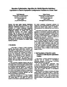
MEMS Device Design Optimization Problem

Our test problem for the model hierarchy surrogates is a deterministic version of the bistable microelectromechanical system (MEMS) switch design problem presented in Ref. 33. For such bistable switches, the goal is to determine a shape for the switch arms that will reliably exhibit the desired force-displacement characteristics despite variability in the manufacturing process. The deterministic version of this problem seeks an optimal design with the uncertain manufacturing parameters fixed at their mean values. The problem consists of 13 geometric design variables (d) and three nonlinear constraints on minimum force, displacement, and maximum stress. An example force-displacement curve for this switch is shown in Fig. 6. Positions E1 and E3 are stable equilibrium points and E2 is unstable. The force required to actuate the switch by displacing the switch arms from E1 through E2 and have them come to rest at E3 is denoted by Fmax . The force required to pass the switch arms from position E3 back through E2 to E1 is denoted as Fmin . The design problem we are interested in solving can be formulated as follows: max s.t.

Fmax (d) E2 (d) Smax (d) Fmin (d)

≤ 8 ≤ 3000 = −5.

(30)

where Smax is the maximum material stress and Fmax , Fmin , and E2 are as described above. To compute the quantities of interest, finite element analysis of the switch is performed using the Aria simulation code34 developed at Sandia National Laboratories. The model hierarchy for this problem arises from the finite element analysis of the switch. Different grid sizes (h-refinement) and element orders (p-refinement) lead to low-fidelity and high-fidelity models. For the experiments presented here, 160 linear elements (resulting in 205 nodes) were used for the low-fidelity model and 1200 quadratic elements (5061 nodes) were used for the high fidelity model. As a simple gauge of the complexity of the different models, Table 7 shows the average times (over 10 runs) for performing a single function evaluation for these models. The times reported here are for those on a single 3.06 GHz Xenon processor with 4 GB of RAM. These times suggest that on average, the cost of a high-fidelity function 15 of 20 American Institute of Aeronautics and Astronautics

Table 6. Example CUTE problems for testing SBO using data fit surrogates. The strategy labels indicate original (OR), basic Lagrangian (BL), or augmented Lagrangian (AL) approximate subproblem; original (OR), linearized (LI), or no (NO) constraints; global (G), local (L), or TANA-3 (T) surrogates, augmented Lagrangian (AL), basic Lagrangian (BL), adaptive penalty (AP), or basic penalty (BP) merit function, filter (F) or trust region ratio (R) acceptance logic, and no relaxation (N) or constraint relaxation (C). A star (*) indicates all choices produced the same results.

CUTE Reference AVGASA

Short Description Academic problem

Var. 6

Ineq. Constr. 6

Eq. Constr. 0

CSFI1

Continuous caster design

5

2

2

CSFI2

Continuous caster design

5

2

2

FCCU

Fluid catalytic cracker modeling

19

0

8

HEART8

Dipole model of the heart

8

0

8

HIMMELBK

Nonlinear blending

24

14

0

HS073

Optimal cattle feeding

4

2

1

HS087

Electrical networks

9

0

4

HS093

Transformer design

6

2

0

HS100

Academic problem

7

4

0

HS114

Alkylation

10

8

3

HS116

Membrane separation

13

15

0

LEWISPOL

Number theory

6

0

9

PENTAGON

Applied geometry

6

12

0

Best Strategies OR-OR-T-**-R-* OR-OR-L-**-R-* OR-OR-L-BL-F-* OR-OR-L-AP-R-C OR-OR-L-AP-R-N OR-OR-L-AP-R-N OR-OR-T-AL-R-N AL-OR-T-AL-R-N AL-OR-T-AL-R-C OR-OR-T-**-R-N OR-OR-T-**-F-N OR-OR-L-**-R-N OR-OR-T-AL-R-N OR-OR-T-AL-F-N OR-OR-T-*P-*-N OR-LI-T-BL-R-N OR-LI-T-AP-R-N OR-OR-L-AP-R-N OR-LI-*-*P-R-N OR-LI-*-*P-R-C OR-LI-*-BL-R-N OR-OR-T-BP-R-N OR-OR-L-AP-R-N OR-OR-L-AL-F-N OR-OR-T-*L-F-N OR-OR-T-BL-F-C OR-OR-T-AL-F-C OR-OR-T-BP-R-* OR-OR-T-BP-F-* OR-OR-T-BL-R-N OR-OR-T-BL-F-C OR-OR-T-BL-F-N OR-OR-L-AP-F-N OR-OR-L-AP-R-C OR-OR-L-BP-R-C OR-OR-L-AP-R-N OR-OR-T-**-*-N OR-OR-L-**-R-N OR-OR-L-**-F-N OR-OR-L-AL-R-N OR-OR-L-BP-R-N OR-OR-L-BP-R-C

16 of 20 American Institute of Aeronautics and Astronautics

Function Evaluations 59 (348) 75 (419) 84 (358) 45 (226) 47 (194) 48 (257) 44 (404) 44 (534) 44 (647) 72 (543) 79 (534) 80 (532) 83 (997) 88 (1012) 91 (1289) 27 (94) 31 (102) 42 (261) 24 (48) 24 (55) 27 (52) 41 (219) 65 (325) 70 (285) 66 (404) 164 (1137) 573 (2864) 47 (457) 50 (414) 52 (425) 67 (724) 71 (249) 75 (298) 39 (106) 40 (288) 42 (65) 23 (63) 38 (298) 44 (354) 40 (281) 40 (281) 41 (271)

Fmax

0 Fmin E1

E2

E3

Figure 6. Example Force-displacement curve for the MEMS device design optimization problem.

evaluation is about 38–39 times as expensive as that for the low-fidelity model for the two models used in our tests. Table 7. Average function evaluation times (seconds) for different models of the finite element analysis of the MEMS bistable switch.

Element Type Linear Quadratic

Number of Elements 160 1200 5.0465 39.414 24.757 194.98

The NPSOL35 and DOT36 optimization codes were used for optimizing the high-fidelity models in singlefidelity approaches and the corrected low-fidelity surrogate models in SBO approaches. Finite differences with steps of 10−3 were used for approximating the derivative information required for the minimization in both approaches and for the first-order additive corrections used in SBO. The initial design was provided by a MEMS design analyst as a useful starting point, but was initially infeasible with respect to the equality constraint involving Fmin in Eq. 30. Convergence tolerances have slightly different meanings in the SBO strategy, NPSOL, and DOT, so we present our findings as plots of the iterates determined by each algorithm for comparison. In all of the optimization runs, the inequality constraints E2 and Smax were inactive. Figure 7(a) shows the relative error of Fmin with respect to the target value of −5 for iterates computed by NPSOL in single-fidelity and multifidelity SBO approaches. NPSOL single-fidelity approaches using either forward differences computed by DAKOTA or a mix of forward and central differences computing internally (see Ref. 35 for a description of how these are determined) were unable to locate a feasible design. The NPSOL single-fidelity approach using forward differences did not yield much progress from the initial design, and thus the more successful of the two approaches is shown. The SBO multifidelity approach, on the other hand, did converge successfully to a feasible design using only forward differences. The horizontal axes in Fig. 7 represent the amount of high-fidelity work units performed by each method. A work unit is the equivalent of a single high-fidelity function evaluation in terms of the times presented in Table 7. Thus, the amount of work performed in the SBO strategy is given by WSBO = nH + 38 × nL

(31)

where nH and nL are the numbers of high-fidelity and low-fidelity function evaluations performed, respectively. Figure 7(a) suggests the SBO is able to solve the problem more quickly and reliably than NPSOL and using less accurate derivatives. For problems such as this one, where function evaluations are very costly for the high-fidelity model, the use of forward over central differences is preferred. Figure 7(b) shows the plot of the relative error in Fmin when using DOT for single-fidelity and multifidelity SBO approaches. Again, central difference results are presented for single-fidelity DOT, since the use of forward differences did not yield a feasible design. The DOT multifidelity SBO approach with forward differences 17 of 20 American Institute of Aeronautics and Astronautics

1

3

10

10

SBO−Dakota FD Single−NPSOL CD

SBO−Dakota FD Single−DOT CD

2 0

10

1

Fmin Relative Error

Fmin Relative Error

10

10

0

10

−1

10

−2

10

−1

10

−2

10

−3

10

−4

10

−3

10

−4

10

−5

0

50

100

150

200

250

10

300

0

20

40

High Fidelity Work Units

60

80

100

120

140

160

180

High Fidelity Work Units

(a) NPSOL

(b) DOT

Figure 7. Relative error of the MEMS design constraint Fmin with respect to the target value of −5 using NPSOL and DOT for optimizing the low-fidelity surrogates in the SBO strategy (blue) and the high-fidelity model in the single model strategy.

and the single-fidelity approach using internally-computed central differences converged to the same locally optimal design, within the numerical tolerances determined by each algorithm. These results again suggest that the SBO strategy is able to produce a locally optimal solution with less work.

IV.

Conclusions

This paper presents and compares a number of algorithmic variations for surrogate-based optimization, including approximate subproblem formulations, merit function selections, iterate acceptance logic options, constraint relaxation approaches, and convergence assessment techniques. In addition, tailoring of these techniques for data fit, multifidelity, and ROM cases is discussed. One research theme is the streamlining of the SBO process through the elimination (or reduction) of requirements for external management of penalty parameters and Lagrange multipliers. Not only does this simplify, but it can also improve performance through elimination of additional SBO cycles needed to converge penalty parameter and Lagrange multiplier estimates. Use of the direct surrogate approach for the approximate subproblems and use of a filter method for iterate acceptance tests moves the SBO algorithm toward the state of being penalty- and multiplier-free. Extensive computational results are presented for SBO with local, multipoint, and global data fit surrogates applied to a number of algebraic test problems (Barnes and selected CUTE test problems). Initial results indicate that the direct surrogate approach, combined with an augmented Lagrangian merit function, is the most efficient and reliable technique developed to this point. This technique is carried forward for an engineering design study in the multifidelity optimization of microelectromechanical systems. The multifidelity technique is shown to result in significant computational savings relative to single-fidelity approaches. The SBO performance results in this paper reflect an ongoing work in progress. Future work will include investigation of fully penalty- and multiplier-free approaches which define a filter-based merit function, constraint relaxation approaches which link the relationship between optimal and feasible directions to the homotopy control parameters, and careful investigation of current SBO algorithm failures observed for alternative subproblem formulations.

V.

Acknowledgments

This work was supported in part by the Applied Mathematics Research program of the Office of Advanced Scientific Computing Research of DOE’s Office of Science. The authors gratefully acknowledge the assistance of Dr. Victor Perez of GE CIAT in sharing his experiences in surrogate-based optimization during his 20032004 postdoctoral appointment with the Computer Science Research Institute (CSRI) at Sandia National Laboratories. In addition, the 2005 CSRI visits of Theresa Robinson (MIT) and Gary Weickum (CU Boulder) have influenced our approaches for multifidelity and reduced-order model surrogates, respectively.

18 of 20 American Institute of Aeronautics and Astronautics

References 1 Schmit Jr., L. A. and Miura, H., “Approximation Concepts for Efficient Structural Synthesis,” Tech. Rep. NASA CR-2552, NASA, March 1976. 2 Barthelemy, J. F. M. and Haftka, R. T., “Chapter 4. Function Approximations,” Structural Optimization: Status and Promise, edited by M. P. Kamat, Vol. 150 of Progress in Astronautics and Aeronautics, AIAA, Washington, DC, 1993. 3 Sobieszczanski-Sobieski, J. and Haftka, R. T., “Multidisciplinary Aerospace Design Optimization: Survey of Recent Developments,” Structural Optimization, Vol. 14, No. 1, 1997, pp. 1–23. 4 Alexandrov, N. M., Dennis Jr., J. E., Lewis, R. M., and Torczon, V., “A Trust Region Framework for Managing the Use of Approximation Models in Optimization,” Structural Optimization, Vol. 15, 1998, pp. 6–23. 5 Giunta, A. A. and Eldred, M. S., “Implementation of a Trust Region Model Management Strategy in the DAKOTA Optimization Toolkit,” Proceedings of the 8th AIAA/USAF/NASA/ISSMO Symposium on Multidisciplinary Analysis and Optimization, Long Beach, CA, September 6-8, 2000, AIAA Paper 2000-4935. 6 Fadel, G. M., Riley, M. F., and Barthelemy, J.-F. M., “Two Point Exponential Approximation Method for Structural Optimization,” Structural Optimization, Vol. 2, No. 2, 1990, pp. 117–124. 7 Xu, S. and Grandhi, R. V., “Effective Two-Point Function Approximation for Design Optimization,” AIAA Journal, Vol. 36, No. 12, 1998, pp. 2269–2275. 8 Rodriguez, J. F., Renaud, J. E., and Watson, L. T., “Convergence of Trust Region Augmented Lagrangian Methods Using Variable Fidelity Approximation Data,” Structural Optimization, Vol. 15, 1998, pp. 1–7. 9 Alexandrov, N. M., Lewis, R. M., Gumbert, C. R., Green, L. L., and Newman, P. A., “Optimization with VariableFidelity Models Applied to Wing Design,” Proceedings of the 38th Aerospace Sciences Meeting and Exhibit, Reno, NV, 2000, AIAA Paper 2000-0841. 10 Vanderplaats, G. N., Numerical Optimization Techniques for Engineering Design: With Applications, McGraw–Hill, New York, 1984. 11 Nocedal, J. and Wright, S. J., Numerical Optimization, Springer, New York, 1999. 12 Gill, P. E., Murray, W., and Wright, M. H., Practical Optimization, Academic Press, New York, 1981. 13 P´ erez, V. M., Renaud, J. E., and Watson, L. T., “An Interior-Point Sequetial Approximation Optimization Methodology,” Structural and Multidisciplinary Optimization, Vol. 27, No. 5, July 2004, pp. 360–370. 14 Omojokun, E. O., Trust Region Algorithms for Optimization with Nonlinear Equality and Inequality Constraints, Ph.D. thesis, University of Colorado, Boulder, Colorado, 1989. 15 Celis, M. R., Dennis, J. E., and Tapia, R. A., “A Trust Region Strategy for Nonlinear Equality Constrained Optimization,” Numerical Optimization 1984 , edited by P. T. Boggs, R. H. Byrd, and R. B. Schnabel, SIAM, Philadelphia, USA, 1985, pp. 71–82. 16 Wujek, B. A. and Renaud, J. E., “New Adaptive Move-Limit Management Strategy for Approximate Optimization, Part 1,” AIAA Journal, Vol. 36, No. 10, 1998, pp. 1911–1921. 17 Wujek, B. A. and Renaud, J. E., “New Adaptive Move-Limit Management Strategy for Approximate Optimization, Part 2,” AIAA Journal, Vol. 36, No. 10, 1998, pp. 1922–1934. 18 Fletcher, R., Leyffer, S., and Toint, P. L., “On the Global Convergence of a Filter-SQP Algorithm,” SIAM J. Optim., Vol. 13, No. 1, 2002, pp. 44–59. 19 Conn, A. R., Gould, N. I. M., and Toint, P. L., Trust-Region Methods, MPS-SIAM Series on Optimization, SIAM-MPS, Philadelphia, 2000. 20 Lawson, C. L. and Hanson, R. J., Solving Least Squares Problems, Prentice–Hall, 1974. 21 P´ erez, V. M., Eldred, M. S., , and Renaud, J. E., “Solving the Infeasible Trust-Region Problem Using Approximations,” Proceedings of the 10th AIAA/ISSMO Multidisciplinary Analysis and Optimization Conference, Albany, NY, Aug. 30–Sept. 1, 2004, AIAA Paper 2004-4312. 22 Haftka, R. T., “Combining Global and Local Approximations,” AIAA Journal, Vol. 29, No. 9, 1991, pp. 1523–1525. 23 Lewis, R. M. and Nash, S. N., “A Multigrid Approach to the Optimization of Systems Governed by Differential Equations,” 8th AIAA/USAF/NASA/ISSMO Symposium on Multidisciplinary Analysis and Optimization, Long Beach, CA, 2000, AIAA Paper 2000-4890. 24 Eldred, M. S., Giunta, A. A., and Collis, S. S., “Second-Order Corrections for Surrogate-Based Optimization with Model Hierarchies,” Proceedings of the 10th AIAA/ISSMO Multidisciplinary Analysis and Optimization Conference, Albany, NY,, Aug. 30–Sept. 1, 2004, AIAA Paper 2004-4457. 25 P´ erez, V. M., Renaud, J. E., and Watson, L. T., “Reduced Sampling for Construction of Quadratic Response Surface Approximations Using Adaptive Experimental Design,” Proceedings of the 43rd AIAA/ASME/ASCE/AHS/ASC Structures, Sttural Dynamics, and Materials Conference, Denver, CO, April 22-25, 2002, AIAA Paper 2002-1587. 26 Robinson, T. D., Eldred, M. S., Willcox, K. E., and Haimes, R., “Strategies for Multifidelity Optimization with Variable Dimensional Hierarchical Models,” Proceedings of the 47th AIAA/ASME/ASCE/AHS/ASC Structures, Structural Dynamics, and Materials Conference (2nd AIAA Multidisciplinary Design Optimization Specialist Conference), Newport, RI, May 1–4, 2006, AIAA Paper 2006-1819. 27 Robinson, T. D., Willcox, K. E., Eldred, M. S., and Haimes, R., “Multifidelity Optimization for Variable-Complexity Design,” Proceedings of the 11th AIAA/ISSMO Multidisciplinary Analysis and Optimization Conference, Portsmouth, VA, September 6–8, 2006, AIAA Paper 2006-7114. 28 Weickum, G., Eldred, M. S., and Maute, K., “Multi-point Extended Reduced Order Modeling For Design Optimization and Uncertainty Analysis,” Proceedings of the 47th AIAA/ASME/ASCE/AHS/ASC Structures, Structural Dynamics, and Materials Conference (2nd AIAA Multidisciplinary Design Optimization Specialist Conference), Newport, RI, May 1–4, 2006, AIAA Paper 2006-2145.

19 of 20 American Institute of Aeronautics and Astronautics

29 Lathauwer, L. D., Moor, B. D., and Vandewalle, J., “A Multilinear Singular Value Decomposition,” SIAM Journal on Matrix Analysis and Applications, Vol. 21, No. 4, 2000, pp. 1253–1278. 30 Eldred, M. S., Giunta, A. A., van Bloemen Waanders, B. G., Wojtkiewicz Jr., S. F., Hart, W. E., and Alleva, M. P., “DAKOTA, A Multilevel Parallel Object-Oriented Framework for Design Optimization, Parameter Estimation, Uncertainty Quantification, and Sensitivity Analysis. Version 3.0 Users Manual.” Tech. Rep. SAND2001-3796, Sandia National Laboratories, April 2002. 31 Wujek, B. A., Automation Enhancements in Multidisciplinary Design Optimization, Ph.D. thesis, Department of Aerospace and Mechanical Engineering, Univ. of Notre Dame, South Bend, IN, July 1997. 32 Bongartz, I., Conn, A. R., Gould, N., and Toint, P., “CUTE: Constrained and Unconstrained Testing Environment,” ACM Transactions on Mathematical Software, Vol. 21, No. 1, 1995, pp. 123–160. 33 Adams, B. A., Eldred, M. S., and Wittwer, J. W., “Reliability-Based Design Optimization for Shape Design of Compliant Micro-Electro-Mechanical Systems,” Proceedings of the 11th AIAA/ISSMO Multidisciplinary Analysis and Optimization Conference, Portsmouth, VA, Sept. 6–Sept. 8, 2006, AIAA Paper 2006-7000. 34 Notz, P. K., Subia, S. R., Hopkins, M. H., and Sackinger, P. A., “A Novel Approach to Solving Highly Coupled Equations in a Dynamic, Extensible and Efficient Way,” Computation Methods for Coupled Problems in Science and Engineering, edited by M. Papadrakakis, E. . Onate, and B. Schrefler, Intl. Center for Num. Meth. in Engng. (CIMNE), Barcelona, Spain, April 2005, p. 129. 35 Gill, P. E., Murray, W., Saunders, M. A., and Wright, M. H., “User’s Guide for NPSOL (Version 4.0): A Fortran Package for Nonlinear Programming,” Tech. Rep. SOL-86-2, System Optimization Laboratory, Stanford University, 1986. 36 Vanderplaats Research and Development, Inc., DOT Users Manual, Version 4.20 , 1995.

20 of 20 American Institute of Aeronautics and Astronautics