all free parameters of the network (weights and biases in our case). ... considering feedforward neural networks, but the use of R2 requires ... the linear regression theory [16]. This is ... does not immediately allow the introduction of the concept.
962
IEEE TRANSACTIONS ON CIRCUITS AND SYSTEMS—I: FUNDAMENTAL THEORY AND APPLICATIONS, VOL. 46, NO. 8, AUGUST 1999
FPE-Based Criteria to Dimension Feedforward Neural Topologies Cesare Alippi, Member, IEEE Examples include reconstructing unknown functions [1], time series forecasting [2], and modeling very complex processes [3]. The determination of a model which approximates a function, given a set of input/output pairs, comprises three distinct phases: model selection (to choose the correct complexity of the model), model parameterization or learning (to determine the parameters of the model), and model validation (to evaluate the generalization ability of the model). The model with the optimal generalization ability is then chosen to solve the function-approximation task. The function-approximation problem has been widely Index Terms— FPE, learning from samples, model selection, addressed in the literature, usually with respect to linear models under the assumption that the function to be learned neural networks. is linear or quasilinear. If this is not the case, the family of approximation models must be extended to include nonlinear NOMENCLATURE models such as neural networks [4]. A number of powerful Neural network parameters vector. neural techniques have been developed, such as radial-basis Trained parameters vector. functions [5], [6], mixture of Gaussians [7], feedforward Optimal parameters vector. [8], and recurrent [9] topologies. Training error function. Several criteria have been suggested to select an approError function. priate neural topology by reducing/optimizing the number of Number of training data. neurons/weights in the network (e.g., optimization based on Training data set. spectral decomposition [10], covariance matrix [11], optimal Training pair. brain damage (OBD) [12], surgeon (OBS) [13], and growing Neural network characterized by algorithms [14]). For these methods, model selection is carried Difference between the real value and out by evaluating the performance of different topologies on a new set of examples (crossvalidation). The best model is the the neural output one minimizing the generalization error on the crossvalidation covariance matrix of set. Unfortunately, crossvalidation presents a serious disadvanGradient of tage, especially when a limited data set is available. Saving Hessian of examples to crossvalidate a model reduces the data available Moore-Penrose pseudoinverse of for configuring the parameters (thus impairing the efficiency of gradient w.r.t Orthogonal projector onto the column learning). In such a case, all data should be used for training, thereby making it necessary for the model selection and valispace of dation process to use criteria which estimate the generalization Moody’s effective number of ability of the neural model from the training data itself. parameters. Of particular relevance, among criteria following this prinAlippi’s effective number of ciple, are the generalized prediction error (GPE) [8] and the parameters. network information criterion (NIC) [15]. In this paper, we empirical average of introduce the final prediction error biased (FPEB) criterion which extends the final prediction error (FPE) [16] to the case I. INTRODUCTION of biased models. EARNING an input–output relationship from a set of GPE provides a trivial model selection in noise-free value pairs is a fundamental problem in many fields. applications by selecting the model with the minimal training Manuscript received November 15, 1995; revised September 24, 1998. This error. This procedure is not correct if the number of training paper was recommended by Associate Editor A. Kuh. pairs is small. This limitation is solved by FPEB, which The author is with the Dipartimento di Elettronica e Informazione, Politecintroduces a correction term which is a function of the nico di Milano, 20133 Milano, Italy. Publisher Item Identifier S 1057-7122(99)06358-8. number of training pairs. Abstract—This paper deals with the problem of dimensioning a feedforward neural network to learn an unknown function from input/output pairs. The ultimate goal is to tune the complexity of the neural model with the information present in the training set and to estimate its performance without needing new data for cross-validation. For generality, it is not assumed that the unknown function belongs to the family of neural models. A generalization of the final prediction error to biased models is provided, which can be applied to learn unknown functions both in noise free and noise affected applications. This is based on a new definition of the effective number of parameters used by the neural model to fit the data. New criteria for model selection are introduced and compared with the generalized prediction error and the network information criteria.
L
1057–7122/99$10.00 1999 IEEE
ALIPPI: FPE-BASED CRITERIA
963
FPEB differs from NIC in that FPEB distinguishes between noise-free and noise-affected cases to take advantage of a priori information. It is always computationally feasible, even when NIC is ill-conditioned, and considers an early stopping strategy to limit overtraining effects (overfitting caused by the learning phase) in overdimensioned networks. The problem of learning from examples can be formalized be the unknown as follows. Let the set containing the pairs function to be learned and (1.1) and generated drawn from a stationary density function according to the classical signal-plus-noise model (1.2) is the generic actual measurable output, In other words, corrupted by an independent and identically distributed (i.i.d.) which is generally noise with zero mean and a variance unknown. which best approximates Our goal is to find the function given (1.1) and a loss criterion [e.g., a mean square error (MSE)]. The search for the best approximating function is carried out within a hierarchical model structure . The model considered in this paper contains structure inputs, two-layered feedforward neural networks with hidden units (characterized by a nonlinear differentiable activation function, e.g., a sigmoidal-like function), and a single linear output. The interest for such models derives from the fact that, under weak hypotheses, they are universal function is completely approximators [17]. Each element defined by a column vector of parameters , which contains all free parameters of the network (weights and biases in our case). We will assume that the -dimensional vector differentiable manifold of parameters (if belongs to a the neural network is fully connected between layers then ). The model corresponding to a particular will be denoted . We say that is biased if there does . As a consequence, even in not exist a such that the best case when the learning process provides the optimal (see approximating function , we have that also [18] for a detailed analysis of the bias/variance dilemma). We consider as a simple example of model bias the problem defined in the of learning the noise-free function interval. We choose to be the MSE tending to infinity, with subject to a uniform distribution and the model family . The best approximating function is such that . In this paper we adopt (1.3) as the general error-based criterion for configuring the neural parameters
should converge to an optimal parameter configuration (for which ) yet to be defined. The structure of this paper is as follows. Section II investiand by describing the gates the asymptotic behaviors of elements to which the sequences converge. The general criterion is derived by considering asymptotic results and is tailored to neural networks. The section ends with a brief description of Moody’s GPE. In Section III, results are and we obtain the specialized to the case where FPEB. On the basis of the effective number of parameters, the criterion is then refined to take advantage of a priori information, namely, whether the application is noise free or not. Relationships and differences between FPEB, GPE, and NIC are derived. Finally, in Section IV, the effectiveness of the method is demonstrated on examples of learning nonlinear functions. II. THE GENERAL CRITERION SELECTION AND VALIDATION
FOR
A. Extending Asymptotic Results to Neural Networks Let us define the function
to be the subset of point(s) minimizing (2.1)
evaluated with respect to the probability density function under the hypothesis of i.i.d. inputs. We might interpret as the best average approximation of given and . is such that [19] The relationship between and tends to infinity, converges R1: when uniformly to zero with probability 1 in . This convergence result implies that the set of accumulation are, respectively, the points of local/global minima of points of local/global minima of . Several important results in system identification are based on the asymptotic relationships between points minimizing (1.3) and those minimizing (2.1). Results on convergence and rapidity of convergence are well known under the strong hypothesis that the true system belongs to the model family [16] and, more specifically, to linear models. Results (valid for modeling dynamical systems) have been extended in [20] and [21] to cover the general case where the system does not belong to the model. Now, by assuming that there exists a and denoting with the Hessian unique global minimum matrix (obtained by differentiating twice with respect to ), it has been proved [19] that: (where is the identity matrix and ), then R2: if as tends to infinity and, for a sufficiently , is asymptotically normal (AsN) with large covariance matrix zero mean and (2.2)
(1.3) where ) and (1.3) with dependent reasonable
is a discrepancy or error function (e.g. with . Minimization of a learning procedure will provide a minimum , . As a consequence, it seems on the given tends to infinity, that as the number of pairs
where (2.3) (2.4) It can easily be proved that R1 and R2 still hold when considering feedforward neural networks, but the use of R2 requires some additional care. The assumption of a unique
964
IEEE TRANSACTIONS ON CIRCUITS AND SYSTEMS—I: FUNDAMENTAL THEORY AND APPLICATIONS, VOL. 46, NO. 8, AUGUST 1999
point for in R2 is intended to confine the analysis to the to which converges. In any case, it neighborhood of should be noted that being in different global minima will not modify the behavior of the entities present in (1.3) and (2.1). to be positive A second strong hypothesis of R2 requires definite in the neighborhood of . If there are isolated minima (i.e. for each of which there exists a safe neighborhood satisfying the positive definite condition), then R2 still holds. is singular, we cannot obtain On the other hand, when the inverse needed in (2.3). The problem can be overcome by [30], considering the Moore–Penrose pseudoinverse [31] and we can extend (2.3) as
model (which in the following for ease of notation will be indicated as ) is to consider how the estimate obtained performs on the average (2.6) We can prove that the following relationships hold: (2.7) (2.8) is the matrix trace (see Appendix B for the proof). where , obtained from (2.8) in (2.7), expression By substituting (2.6) can be approximated as
(2.5) is an idemwhere potent matrix. The pseudoinverse is the same as the inverse is nonsingular. In such a case, becomes the when identity matrix and (2.5) coincides with (2.3). The proof is given in Appendix A. Such an extension is relevant, since it (or allows the learning of functions from real data where its estimate) is often singular (see Section IV). A second aspect to be considered is the effect of training time in estimating the parameter vector in overdimensioned networks (we do not know a priori whether the chosen network topology is overdimensioned to the application). This problem does not arise in linear systems where no is training procedures are necessary and the best estimate generally simply computed offline in a single step according to the linear regression theory [16]. This is not the case in neural networks where the parameter configuration evolves during training (being updated by the learning algorithm) and, in a , which long training run, we have that . This might be far from being a good estimate of any problem has also been observed in [22]. Such a behavior is common with overdimensioned networks where overtraining effects are evident (see Section IV). The is reached in correspondence with a finite best estimate of . To keep the effect of overtraining training time under control, the stopping point for the training phase should be carefully determined (e.g., by evaluating the network’s performance on the test set [22]). If, however, no test sets are available because of the shortage of data, then we should also solve this problem. This will be done in Section III where (and therefore a strategy is implemented to determine the correct to be considered). A further problem to be analyzed is the local minima issue which can be experimentally overcome by using suitable learning algorithms and stochastic minimization procedures such as simulated annealing or genetic algorithms which guarantee to reach a global minimum with probability one (even if these methods are often computationally impractical). B. The Criterion The classical derivation [16] may now be followed by introducing a figure of merit which takes into account the complexity of a model. A natural criterion to validate a given
(2.9) Expression (2.9) is of fundamental importance and needs to be interpreted both under the validation and the selection aspects. Validation Aspect: Expression (2.9) states that the averaged expected performance of the model is approximately the sum of the expected loss criterion and a second term, depending on the characteristics of the noise and the sensitivity of the estimate with respect to the parameters. Expression (2.9), once , validates it by providing a given a trained model measure of its generalization ability. Selection Aspect: Expression (2.9) underlines the compromise between the model complexity and training error performances. Obviously, the balance depends on the current trained model. It is well known that by increasing the complexity of the model, the training error will decrease. However, the second term of (2.9), being the trace of a matrix of order (and therefore dependent on the model complexity), increases. The optimal model (selection aspect) is then the of for which , element namely, the model minimizing the generalization error. If a single run is taken into account then, as with the classic with analysis, we can replace the expectation of the only observation we have (2.10) Due to the simplification, all criteria coming from (2.10) provide only an approximation of the generalization ability of the model and, as a consequence, limit the model validation in the following analysis. Fortunately, the introduced approximation does not impair the effectiveness of model selection, at least structure, as proved in [15]. There, the for the considered authors, by extending results given in [23], provide the NIC criterion formally similar to (2.10). In its simple form, NIC does not immediately allow the introduction of the concept of an effective number of parameters (namely the effective number of degrees of freedom used by the model to solve the approximating task). However, in the case of additive noise and a MSE discrepancy function, it can be shown to be related to GPE, which does allow for such a concept. Whenever the network degenerates to a submodel [15], the effective number of parameters is defined by the limit
ALIPPI: FPE-BASED CRITERIA
965
case when tends to a critical value (which, although it is theoretically correct, we experimentally determined to be impractical from the application point of view). Furthermore, NIC may be ill conditioned when the Hessian is singular, thus impairing the effectiveness of the criterion. Finally, NIC is evaluated in correspondence with , which is determined during the long training run. We already indicated that is not necessarily a good estimate of . The criterion proposed in this paper attempts to resolve such limitations. C. A Different Approach: The Generalized Prediction Error An interesting criterion for model selection and validation different from (2.6) has been suggested in [8] where the author introduces the prediction risk for training sets of size , with input density equal to the empirical density defined by the available training set (2.11) inputs are held fixed but the For such training sets, the ’s may vary according to the conditional probability density . The criterion is then defined as the expected validation set error for validation sets of size , in which the unknown input density is replaced with that of the training set . The criterion becomes (2.12) is the weight decay [25] and the Moody’s where effective number of parameters. (2.12) generalizes the wellknown relationship valid for linear systems [24] to nonlinear and biased models. In particular, for the case of the signal. plus-noise model of expression (1.1), we have that Finally, the GPE becomes (2.13)
GPE
In all subsequent analyses we will focus the attention on the MSE loss criterion (3.3) The structure of the section is as follows. In Section III-A, the final prediction error for biased models FPEB is introduced. Different criteria can then be derived from the general one by exploiting a priori knowledge (e.g., by knowing that data are noise free). First, the criterion is specialized to the case of pure punctual bias, as happens when data are not affected by noise. The goal is to approximate a deterministic function. Then, to cope with the fact that, in general, the punctual bias is unknown (data are in this case affected by noise), we consider an approximation which treats the punctual bias as a random variable. This last approximation, even if particularly appealing since it provides a criterion formally similar to FPE, is a priori not correct because the bias is deterministic. By relaxing this last assumption, the correct criterion may be finally obtained by directly deriving it from the general one. In Section III-B, it will be demonstrated that GPE may be related to FPEB. Finally, in Section III-C, we will analyze the impact of training time on the proposed criteria. A. Evaluating the FPEB , we have to adapt the Having chosen a loss function general criterion to it. This requires computation of the trace term present in (2.10). To this end, remembering that and by indicating (3.4) of the error as the column vector of partial derivatives with respect to the generic th parameter component, the matrix of (2.4) can be rewritten as (3.5)
where (2.14) is the Hessian of the objective function and matrix of the derivatives of the training error. III. FPEB: EXTENDING FPE
TO
is the
BIASED MODELS
In the following, we consider the case in which a sufficiently is given, thus making large but finite number of data effective results given in previous analyses. To take into account the model bias, we must refine the signal-plus-noise as the sum of two terms: model of (1.2) by considering and the distortion function the approximating function (3.1) By invoking R1, when
with
Now, by remembering that we obtain that
and
are i.i.d. random variables, (3.6) (3.7)
We next compute
By differentiating (2.1) twice
tends to infinity, (3.1) becomes (3.2) (3.8)
We define
to be the punctual bias in
.
966
IEEE TRANSACTIONS ON CIRCUITS AND SYSTEMS—I: FUNDAMENTAL THEORY AND APPLICATIONS, VOL. 46, NO. 8, AUGUST 1999
all terms being evaluated at . If this is extended to the general may be singular, the trace term present in case where (2.10) can be rewritten as (3.9) (3.10) We define to be the effective number of parameters used by ) the model to fit the data (the rank is full whenever to be a virtual variance associated with the bias. If and (as may happen during training) we should consider instead of . Finally, we can rewrite (2.10) as
(3.11) For large we can substitute in (3.8) the expectation with its empirical value (now evaluated at ) and an estimate of the effective number of parameters can be computed as (3.12)
(3.13) evaluated at . We can further approximate (3.12) to reduce the computational complexity in the evaluation of by considering the quasi-Newton Hessian [i.e., neglecting the second term in becomes the approximated (3.8) and, therefore, in (3.13)]: and the approximated effective number of parameters is
approximators [18]. The second term in (3.13) may also become null with reduced in overdimensioned models if the network overfits the training data in the long training run (see results of Section IV). 1) The Criterion in the Noise-Free Case: Let us now compare (2.12) with (3.11). Whenever the process generating the , the model selection, as data is not affected by noise suggested by Moody [(2.12)], is unrealistic since it is based only on the training error. Equation (3.11) provides a more robust model selection by considering a corrective term, which depends on the complexity of the model and the number of data samples. The criterion in the pure bias case directly derives from (3.11) (3.15)
FPEB
where the effective number of parameters is given either in comes from (3.10) by substituting (3.12) or (3.14) and expectations with the empirical quantities of (3.7) and (3.13). It should be noted that, in a noise-free case, we simply have : a known quantity. , as defined in (3.3), As a simple example let us consider interval, with examples uniformly extracted from the and the model family . . From We have seen that the best approximation is and therefore, from (3.7) (3.4) we have that . From (3.12) and . Equation (3.15), therefore, finally provides the criterion FPEB 2) The Criterion in the Noise-Plus-Bias Case: In the case of the noise is of noise plus distortion, if the variance known, the analysis is straightforward and we have to add to criterion (3.15). Conversely, if the variance of the noise is unknown, it must be estimated. By definition, we have that
(3.14) The effective number of parameters as defined in (3.14) has also been suggested in [26] under the hypothesis of a nonsingular quasi-Newton Hessian. Unfortunately, this is not the case in real applications, where the matrix is generally singular [see also observations following (2.10)]. To overcome such problems, different authors (see [27] for instance) evaluate the effective number of parameters by counting the number of non-null weights and biases. This procedure is definitely not correct and either (3.12) or (3.14) should be used. Moreover, since (3.14) does not always provide a good approximation of the effective number of parameters, (3.12) should be used in preference. The two entities coincide when the term given in (3.13) is null. This happens when dealing with linear models or when the error surface has a relatively constant curvature in the neighborhood and/or the network fits the data well. tends to infinity, then If the punctual bias is null when and we say that the real function to be approximated . In a noise-free environment this always almost belongs to happens by allowing the number of hidden units to increase freely, since the chosen neural models are universal function
(3.16) . By considering (2.8) with terms with coming from (3.10) and (3.16), we have that (3.17) and, therefore, the estimate
becomes (3.18)
By substituting (3.18) in (3.11), we obtain the expression for the criterion in the noise-plus-bias case
FPE
(3.19)
where FPE is the final prediction error term structurally similar to the well-known FPE for unbiased models. Even if the expression is similar to FPE, it should be noted that now
ALIPPI: FPE-BASED CRITERIA
967
contains also the bias contribution (and thus FPE FPE). When grows indefinitely, the training error becomes a good estimate of the generalization error. The criterion suggested in (3.19) relies on the hypothesis and are available or estimable. If this is not the that case, we can address the problem by assuming that also the bias is an i.i.d. variable with zero mean and an unknown variance. The hypothesis relies on the fact that it is reasonable to assume both positive and negative punctual biases with a null expectation and that the effect caused by a punctual bias added to the noise is equivalent to a realization of a different noise with an increased variance [this is due the approximation introduced in (2.9) when deriving (2.10)]. The analysis is now straightforward by simply considering the and additive contribution in the two random variables in (3.1) and (3.2), whose effect is equivalent to a random with zero mean and variance. variable Without presenting all details, we can repeat the procedure accomplished in Section III-A. Briefly, (3.11) becomes
Of course, if is sufficiently large, then the approximation holds because of the law of large numbers. The validity of estimating the covariance matrix from the available data for finite was studied in [16], with respect to ARX models. By using Monte Carlo simulations, the with only 50 data authors obtained good approximations of instances. Similar results were also obtained in [28]. Monte Carlo experiments should also be performed for the case of nonlinear systems, to determine experimentally the impact of on . Experiments presented in Section IV prove finite the validity of the framework outlined in this paper. It seems, therefore, reasonable to assume that we would obtain a good with only a few tens of data. approximation of
(3.20)
and therefore, from (3.10) and (3.16), we obtain a relationship and among
B. Relationships Between Moody’s GPE and FPEB Under Moody’s assumptions, we can estimate the generalization error of (2.10) with the one provided in (2.12) (3.26)
with (3.27) (3.21) As a consequence, the final criterion becomes formally similar to FPE
Equations (3.17) and (3.27) constitute a linear system whose solution gives the estimates (3.28)
FPEB
FPE
(3.22) and, therefore, (3.11) becomes
accounts both for the noise on data and the bias. where The effective number of parameters is, again, either that of expression (3.12) or (3.14). Whenever the model is unbiased, and does not contain any we have that bias contribution and the criterion reduces to FPE. The hypothesis of assuming the bias as a random variable, even if appealing, is not correct from a theoretical point of view and we should consider (3.19). Without specializing the effects of noise and bias, we can still derive from (2.10) a criterion formally similar to NIC. By substituting (2.5) in (2.10) and expectations with empirical quantities, the criterion becomes FPEB
(3.23)
where
GPE
(3.29)
which is equivalent to the GPE given in (2.13), with (3.28) as the estimate of variance. Finally, we could use the estimates of (3.28) to reformulate (in this case) the FPEB FPEB
FPE
(3.30)
. Equation (3.30) where FPE states that, under Moody’s assumptions, the final prediction error in the biased case is structurally equivalent to FPE , corrected by a factor depending on the effective number of parameters and on the bias degree . C. The Impact of Training Time in the Use of FPEB
(3.24) and (3.25) Once again, the number of parameters used by the model is that of (3.12). The validity of the presented criteria relies on the validity of substituting expectations with empirical values. (or In other words, this is equivalent to assuming that ) can be reasonably estimated from the available data.
In all these criteria, whenever the network is overdimensioned with sufficient degrees of freedom with respect to the decreases asymptotically with given application, the term training epochs. On this basis, we should identify the optimal network as the one obtained after infinite training time. With respect to a simple gradient based procedure, and under the hypothesis that the learning coefficient tends to zero and that the number of training epochs tends to infinity, Amari, in [15], proved that for a sufficiently large training has a Gaussian distribution whose expectation time
968
IEEE TRANSACTIONS ON CIRCUITS AND SYSTEMS—I: FUNDAMENTAL THEORY AND APPLICATIONS, VOL. 46, NO. 8, AUGUST 1999
is a point minimizing with variance proportional to the learning coefficient. The proof is only valid for gradient descent algorithms and does not imply that the best estimate is obtained after infinite training but simply that, with a of resampling training procedure, we will converge to a point . In fact, it is not true that after infinite minimizing training epochs we necessarily end in a good minimum (i.e., may be a bad estimate of ) because of overtraining. We already discussed the issue in observations following (2.5). The problem can be solved by implementing an early stopping strategy based on the effective number of parameters. Experimentally, we have seen that training should be is constant stopped whenever converges and/or or increases. The rationale behind this is that represents the effective number of degrees of freedom used by the model to infer the unknown function from the input/output pairs. evolves during the early stages of training as if it were driven by an internal growing/optimizing algorithm, which provides the appropriate degrees of freedom. Heuristically, is constant or increases, the when converges and training procedure needs to be stopped and, at that time, the , etc.) should be used in the associated entities (e.g., criteria. A different theory, dealing with the determination of the optimal stopping point, has been developed in [32] where belongs to a it has been proven that the optimal point neighborhood of . The two criteria are equivalent since, in such a neighborhood, (2.7), (2.8) and the following relationships are valid.
of hidden neurons decreases, but this strategy provides useful guidelines in reducing the number of models to be considered. Generally, in a few iterations we can identify a small set of candidate topologies containing the optimal one. Training was implemented with an optimized Levenberg–Marquardt learning algorithm. In the rest of the section, we will compare several criteria which are derived from FPE or FPEB, by considering the novel definition of the effective number of parameters. More specifically, the following are the criteria. 1) FPE: the criterion is the well-known FPE for which is the number of nonnull degrees of freedom of the network; 2) FPE1: the criterion is the FPE for which the number of parameters has been evaluated according to (3.14) (we consider the approximated version of ). 3) FPE2: the criterion is the FPE for which the number of parameters has been evaluated according to (3.12) (we consider the correct ). 4) FPEB: the criterion is the one given in (3.15) for the pure bias case and the one in (3.23) for the most general case with the approximated effective number of parameters from (3.14). 5) FPEB2: the criterion is the one given in (3.15) for the pure bias case and the one in (3.23) for the general case with the correct effective number of parameters from (3.12). This criterion is the most accurate one. A. Example 1: A Reduced-Bias Case
IV. LEARNING INPUT/OUTPUT RELATIONSHIPS In this section we apply the criteria proposed above to determine the optimal neural topology in three applications. The first application deals with a smooth function in a noisefree set up. The second application also refers to a noise-free case but, in this example, the function to be learned is quite irregular and the data do not contain sufficient information to properly configure the neural model. In the third application, the function to be learned is affected by noise. Selection of the optimal topology according to FPEB requires the training of several hierarchical models (the hierarchy can be obtained by increasing the number of hidden units). Obviously, the training procedure is time consuming and training a large subset of the model structure may be computationally infeasible. Heuristics can therefore be used to guide the search toward the determination of a reduced subset of models. To this end, two different approaches can be found in [2] and [29]. Here, we implemented the second one. Briefly, instead of training and evaluating the criterion for each different neural topology, we apply an OBD-like technique [25] to connections ending in the output neuron of a strongly overdimensioned topology. The hidden layer complexity can be reduced (thus exploring the hierarchy) by removing the connectio,n after which the increase in MSE is minimized. A new topology is given and the criterion can be applied without requiring a new training phase. This OBD-like process iterates until the number of hidden units is equal to one. The error in estimating the criterion without any effective training increases as the number
Our goal is to approximate the nonlinear function (4.1) For this example, the training set was composed of pairs uniformly extracted from the interval. The function is smooth and the training set rich enough to guarantee that (4.1) almost belongs to the neural model family. No noise was added to the data: this is a pure bias case. The heuristic outlined above was used to consider topologies with hidden units ranging from one to seven. For each neural model we have to apply the training procedure and then compute the criteria. According to the early stopping strategy, we monitored the evolution of the correct and the approximated effective number of parameters during training time. The learning phase lasted for 1000 epochs (each epoch implements two minimizations of the training error). In the indicates the number of hidden units and following plots, the asymptotic value (with respect to the training epochs) assumed by . The evolution of the correct effective number of parameters for each topology of the subset is given in Fig. 1. We can , the network utilizes all immediately see that with the degrees of freedom available, whereas for networks with higher complexity, the effective number of parameters is less hidden neurons we have than the maximum (for weights and biases). The behavior of the models is such that first evolves during the initial with
ALIPPI: FPE-BASED CRITERIA
Fig. 1. The correct effective number of parameters.
Fig. 2. The approximated effective number of parameters.
stages of learning, before reaching a steady state (note that experiment the model degenerated to a model for the with lower complexity). The evolution of the approximated effective number of parameters is given in Fig. 2. term of exThe approximation does not consider the pression (3.13). Since the function almost belongs to the neural model family, after a small number of training epochs we have and the correct and the approximated coincide that (as happens) in the long training run. Comparisons among different criteria are given in Fig. 3 where we indicated the MSE validation for the case with MSEval and MSE training with MSEtr. We can see that, despite the approximation leading to (2.10), FPEB and FBEB2 are reasonable estimates of the MSE validation (evaluated over the whole definition interval) while all other criteria provide a worse estimate. The effective number of parameters and the criteria have been determined with the early stopping strategy suggested in Section III-C. The most accurate criteria are then compared in Fig. 4 for neural models with hidden units varying from one to five. For all models, FPEB2 provided a good estimate of the generalization ability, while all criteria , in full agreement with the selected the model with
969
Fig. 3. Comparing different criteria for the model with
nh = 2.
Fig. 4. Different criteria for the models from one to five hidden units.
validation plot. Actually, there is a very small improvement in performance when increasing the number of hidden units, but we are interested in the smallest model keeping the same performance. The training data (circled), the function to be learned, and the best neural model selected by the criteria are plotted in Fig. 5. B. Example 2: A High-Bias Case In this experiment, we drastically reduced the number of training data to 32 and enlarged the definition interval to . Data was regularly sampled from the function (4.2) and no noise was added. This function is definitely more irregular than the previous one (see Fig. 11). The OBD-like procedure identified the interval from one to ten hidden units. To monitor overtraining effects, we have to track the evolution of the correct (Fig. 6) and the approximated (Fig. 7) effective and increase from number of parameters. In the figures, the bottom to the top of the plots. It can be seen that now there is a difference in the estimated effective number of parameters
970
IEEE TRANSACTIONS ON CIRCUITS AND SYSTEMS—I: FUNDAMENTAL THEORY AND APPLICATIONS, VOL. 46, NO. 8, AUGUST 1999
Fig. 5. The training data, the real function and the best neural model.
Fig. 8. Evolution of the criteria in the long training run for the model with nh 5.
=
Fig. 9. Different criteria for the models from four to nine hidden units. Fig. 6. The correct effective number of parameters.
Fig. 7. The approximated effective number of parameters.
for the case (we have for the correct and for the approximated one in the long training run). Since the network is overdimensioned, the for high values of stopping points suggested by the two estimates are different. For overdimensioned models, the best stopping point is at the early stages of learning where the correct and the approximated effective number of parameters differ. we should, therefore, always consider the correct . In Fig. 8, the evolution of different criteria over the training is plotted on a semilog scale. We time for the case realize, once more, that the FPEB’s provide better estimates of the generalization ability of the model (again there is a discrepancy between FPEB and FPEB2 because of the difference in ). FPE, itself, is always the worst criterion. We determined the best criterion FPEB2 and FPE (the worst one) on different network topologies with hidden units varying from four to nine. Results are given in Fig. 9. FPE selected the model with five hidden units, while FPEB2 selected the one with six. The model with eight hidden units almost provides the same performance (according to the criterion) as the one with six, but it requires a more complex model. On the other
ALIPPI: FPE-BASED CRITERIA
Fig. 10.
971
The training data, the real function, and the best neural model. Fig. 12. The correct effective number of parameters.
Fig. 11.
Overtraining effects for the model with ten hidden units.
hand, the criterion will penalize such a model if the model complexity is overdimensioned with respect to the number of data elements. The selected model is then the one which best solves the performance/model complexity tradeoff according to (3.23), even if this may imply the selection of a model with a high bias (see Fig. 10). Validation results support the selections made and prove the efficacy of estimating the validation error with FPEB2. The best approximation, as suggested by the criterion, is given in Fig. 10 where the training data are circled, the real function of (4.2) is plotted in a continuous line, and the best estimate with a dotted line. If the learning termination point is not correctly selected (e.g., according to the early stopping strategy based on and the criteria), we could easily end up with overtrained networks. An example is the plot of Fig. 11, obtained after only 400 topology. We can see that training epochs for the after too much training is a bad estimate of . C. Example 3: Noise and Bias As a third example, we consider the function (4.3) as suggested in [17]. A set of
’s were uniformly
Fig. 13. Evolution of the criteria in the long training run for the model with nh 4.
=
extracted from the interval and the associated ’s were corrupted with a Gaussian noise with zero mean and variance. We assume that the process generating the data is unknown. Since we do not have a priori knowledge, we have to consider the most general criterion given in (3.23). The same heuristic suggests examination of models with from one to five hidden neurons. As with previous cases, we monitored the evolution of the correct effective number of parameters. Fig. 12 shows the 1–400 training epoch interval for models with from to three hidden units. We can see reaches one after some training that for the case epochs and then it converges by using all the degrees of freedom provided by the model (i.e., four). The model with two hidden units uses only six parameters out of seven, while , decreases and converges to the in the case of steady state with eight parameters out of ten. It is easy to determine the learning termination points for such topologies. The behavior of the most relevant criteria over the training . The behavior run is given in Fig. 13 for the case of the criteria with respect to different neural topologies (from one to five hidden units) are plotted in Fig. 14. We
972
IEEE TRANSACTIONS ON CIRCUITS AND SYSTEMS—I: FUNDAMENTAL THEORY AND APPLICATIONS, VOL. 46, NO. 8, AUGUST 1999
APPENDIX A To calculate the parameter covariance matrix of (2.3) and (2.5) we need to expand around (to which converges) with Taylor and evaluate the (the learning procedure expansion at . Since ends in a minimum) the expansion provides (A.1) where each component of the vector is within a sphere of centred on . radius tends to infinity tends to and In the limit, when converges uniformly to with probability 1 in from R1. Under the regularity hypothesis, this convergence also holds converges to (see [19] for the Hessians and therefore and [20] for the proof). (A.1) thus becomes Fig. 14.
(A.2)
Different criteria for the models from one to five hidden units.
(A.2) constitute a linear system whose Moore–Penrose solution in the mean square sense is [30], [31] (A.3) is an where is the identity matrix, orthogonal projector onto the idempotent matrix , and is an arbitrary -dimensional column/row space of column vector. From simple manipulations and remembering that , we can write that
(A.4)
Fig. 15.
The training data, the real function, and the best neural model.
can see that the networks with two and four hidden units provide the same performance. Since we choose the simplest model when determining the complexity/performance tradeoff, we consider only the network with two hidden units. The best estimate is given in Fig. 15 (training data: circled, real function: continuous line, best approximation: dashed line). V. CONCLUSION In this paper we presented a theoretical framework which provides effective criteria to select and validate neural topologies for learning an unknown function. A generalization of the FPE criterion to biased models has been introduced, which is shown to be related to the one suggested by Moody. The criteria solve problems posed by NIC. This has been achieved by suitably estimating the covariance matrix of the parameters with the Moore–Penrose pseudoinverse by introducing a novel definition of the effective number of parameters and by implementing an early learning termination strategy which helps prevent overtraining.
The second term of (A.4) can be neglected since is asymptotic to , which is null is (see also [15]) and (2.5) is proved. When and we obtain (2.3). nonsingular we have simply that APPENDIX B and are not With respect to (2.6) we note that known, since we do not know the true data. Such quantities will therefore be approximated by using Taylor expansions in the Lagrange notation around the minimum (to which will . Recalling that and evaluating converge) of , we obtain the expansion for (B.1) where radius
is a point whose components lie within a sphere of centered on . We recall that (A.1) holds (B.2)
around , consider We expand given by (B.2), and evaluate the expansion for
as
(B.3)
ALIPPI: FPE-BASED CRITERIA
973
where is a convenient point similar to and . We now take expectations of (B.1) and (B.3) by considering the asymptotic relationships given by R1 and expression (2.2), thus obtaining
(B.4)
(B.5) being recall that
and
the matrix trace. From (2.1) we (B.6)
From (B.1) to (B.6), we obtain finally (B.7) (B.8) from which (2.7) and (2.8) follow by noting that . ACKNOWLEDGMENT The author wishes to thank the reviewers for their insights and fruitful suggestions in early versions of the paper and J. Taylor and Dr. K. Sammut for help in improving its readability. REFERENCES [1] J. Hertz, A. Krogh, and R. G. Palmer, Introduction to the Theory of Neural Computation. Reading, MA: Addison-Wesley, 1991. [2] J. Moody and J. Utans, “Principal architecture selection for neural networks: Application to corporate bond rating prediction,” in Proc. NIPS4, San Mateo, CA, 1992, pp. 683–690. [3] A. G. Parlos, K. T. Chong, and A. F. Atiya, “Application of the recurrent multilayer perceptron in modeling complex process dynamics,” in IEEE Trans. Neural Networks, vol. 5, pp. 255–266, Mar. 1994. [4] M. Stinchombe and H. White, “Approximating and learning unknown mappings using multilayer feed-forward networks with bounded weights,” in Proc. IJCNN’90, 1990, vol. 3, pp. 7–16. [5] F. Girosi, M. Jones, and T. Poggio, “Regularization theory and neural networks architectures,” Neural Computat. 1994, vol. 7, 1995. [6] F. Girosi, M. Jones, and T. Poggio, “Priors, stabilizers and basis functions: From regularization to radial, tensor and additive splines,” Dept. Brain and Cognitive Sciences, MIT, Cambridge, MA, A.I. Memo 1430, 1993. [7] J. L. Marroquin, “Measure fields for function approximation,” , Artificial Intelligence Lab., MIT, Cambridge, MA, A.I. Memo 1433, 1993. [8] J. Moody, “The effective number of parameters: An analysis of generalization and regularization in nonlinear learning systems,” in Proc. NIPS4, San Mateo, CA, 1992, pp. 847–854. [9] IEEE Trans. Neural Networks (Special Issue on Recurrent Networks), vol. 5, pp. 153–337, Mar. 1994. [10] C. Alippi and V. Piuri, “Topological minimization of multi-layered feed-forward neural networks by spectral decomposition,” in Proc. IEEE-IJCNN’92, Beijing, China, Nov. 3–6, 1992. [11] A. S. Weigend and D. E. Rumelhart, “The effective dimension of the space of hidden units,” in Proc. IEEE-IJCNN, Singapore, 1991.
[12] Y. Le Cun, J. S. Denker, and S. A. Solla, “Optimal brain damage,” in Proc. NIPS2, San Mateo, CA, 1990. [13] B. Hassibi and D. G. Stork, “Second order derivative for network pruning: Optimal brain surgeon,” in Proc. NIPS5, San Mateo, CA, 1993. [14] A. Sankar and R. J. Mammone, “Growing and pruning neural trees network,” in IEEE Trans. Comput., vol. 52, pp. 291–299, Mar. 1993. [15] N. Murata, S. Yoshizawa, and S. Amari, “Network information criterion—Determining the number of hidden units for an artificial neural network model,” in IEEE Trans. Neural Networks, vol. 5, pp. 865–872, Nov. 1994. [16] L. Ljung, System Identification, Theory for the User. Englewood Cliffs, NJ: Prentice-Hall, 1987. [17] K. Hornik, M. Stinchombe, and H. White, “Multilayer feedforward networks are universal approximators,” in Neural Networks, vol. 2, 1989. [18] S. Geman, E. Bienenstock, and R. Doursat, “Neural networks and the bias/variance dilemma,” in Neural Comput., vol. 4, pp. 1–58, 1992. [19] L. Ljunga and P. Caines, “Asymptotic normality of prediction error estimators for approximate system models,” in Stochastic, vol. 3, pp. 29–46, 1979. [20] L. Ljung, “Convergence analysis of parametric identification methods,” IEEE Trans. Automat. Contr., vol. AC-23, no. 5, pp. 770–783, 1978. [21] P. Caines, “Stationary linear and nonlinear system identification and prediction set completeness,” IEEE Trans. Automat. Contr., vol. AC-23, no. 4, pp. 583–594, 1978. [22] S. Amari, “Statistical and information-geometrical aspects of neural learning,” in Computational Intelligence: A Dynamic Perspective. New York: IEEE, 1995, pp. 71–82. [23] H. Akaike, “Statistical predictor identification,” in Ann. Inst. Stat. Math., vol. 22, 1970. [24] A. Barron, “Predicted squared error: A criterion for automatic model selection,” in Self-Organizing Methods for Modeling, S. Farlow Ed. New York: Marcel Dekker, 1984. [25] I. Guyon, V. Vapnik, B. Boser, L. Bottou, and S. A. Solla, “Structural of risk minimization for character recognition,” in Proc. NIPS4, 1992. [26] J. Larsen and L. K. Hansen, “Generalization performance of regularised neural network models,” in Proc. Workshop Neural Networks Signal Processing, 4, Piscataway, NJ, 1994, pp. 42–51. [27] M. Norgaard, “Neural network based system identification toolbox for Matlab,” Inst. Automation, Tech. Univ. Denmark, Tech. Rep. 95-E-773, 1995. [28] T. Soderstrom and P. Stoica, “Instrumental variable methods for systems identification,” in Lecture Notes in Control and Information Sciences. New York: Springer-Verlag, 1983. [29] C. Alippi, “Spectral decomposition, Rissanen’s and Akaike’s criteria to select and validate neural structures,” in Proc. World Cong. Neural Networks, Washington, DC, 1995. [30] G. Strang, Linear Algebra and Its Applications. Orlando, FL: Harcourt Brace Jovanovich, 1986. [31] C. R. Rao, Linear Statistical Inference and Its Applications. New York: Wiley, 1973. [32] S. Amari, N. Murata, K. R. Muller, M. Finke, and H. Yang, “Asymptotical statistical theory of overtraining and cross-validation,” in Proc. NIPS8, 1996.
Cesare Alippi (S’92–M’97) received the Dr.Ing. degree in electronic engineering (summa cum laude) and the Ph.D. degree in computer engineering from the Politecnico di Milano, Milano, Italy, in 1990 and 1995, respectively. He is currently an Associate Professor in Computer Science at the Politecnico di Milano and a Research Fellow in the Italian National Research Council. His research interests include neural networks (learning theories, implementation issues and applications), genetic algorithms, nonlinear signal and image processing, and VLIW architectures. His research results have been published in more that 70 technical papers in international journals and conference proceedings.