Inverting feedforward neural networks using linear and nonlinear ...

IEEE TRANSACTIONS ON NEURAL NETWORKS, VOL. 10, NO. 6, NOVEMBER 1999

1271

Inverting Feedforward Neural Networks Using Linear and Nonlinear Programming Bao-Liang Lu, Member, IEEE, Hajime Kita, and Yoshikazu Nishikawa

Abstract—The problem of inverting trained feedforward neural networks is to find the inputs which yield a given output. In general, this problem is an ill-posed problem because the mapping from the output space to the input space is a one-tomany mapping. In this paper, we present a method for dealing with the inverse problem by using mathematical programming techniques. The principal idea behind the method is to formulate the inverse problem as a nonlinear programming (NLP) problem, a separable programming (SP) problem, or a linear programming (LP) problem according to the architectures of networks to be inverted or the types of network inversions to be computed. An important advantage of the method over the existing iterative inversion algorithm is that various designated network inversions of multilayer perceptrons (MLP’s) and radial basis function (RBF) neural networks can be obtained by solving the corresponding SP problems, which can be solved by a modified simplex method, a well-developed and efficient method for solving LP problems. We present several examples to demonstrate the proposed method and the applications of network inversions to examining and improving the generalization performance of trained networks. The results show the effectiveness of the proposed method. Index Terms— Boundary training data, feedforward neural networks, generalization, inverse problem, iterative inversion algorithm, linear programming, neural-network inversions, nonlinear programming, separable programming.

I. INTRODUCTION

T

HE problem of training a feedforward neural network is to determine a number of adjustable parameters or on the basis connection weights, which are denoted by of a set of training data. A trained feedforward neural network can be regarded as a nonlinear mapping from the input space to the output space. Once a feedforward neural network has been trained on a set of training data, all the weights are fixed. Thus the mapping from the input space to the output space is determined. This mapping is referred to as the forward mapping. In general, the forward mapping is a many-toone mapping because each of the desired outputs usually corresponds to several different training inputs in the training set. We express the forward mapping as follows: (1) Manuscript received January 16, 1998; revised October 19, 1998 and June 25, 1999. This work was done in part while the first author was a Ph.D student at the Department of Electrical Engineering, Kyoto University, Kyoto, Japan. B. L. Lu is with the Laboratory for Brain-Operative Device, Brain Science Institute, RIKEN, Saitama, 351-0198, Japan. H. Kita is with the Department of Computational Intelligence and Systems Science, Tokyo Institute of Technology, Yokohama 226-8502, Japan. Y. Nishikawa is with the Faculty of Information Sciences, Osaka Institute of Technology, Hirakata 573-0196, Japan. Publisher Item Identifier S 1045-9227(99)08838-4.

where , , and , , represent the input and output of denotes the fixed weights, and the network, respectively, denotes the forward mapping determined by the architecture of the network. For a given input , it is easy to calculate the corresponding output from (1). In contrast, the problem of inverting a trained feedforward neural network is to find inputs which yield a given output Such inputs are called the network inversions or simply inversions. The mapping from the output space to the input space is referred to as the inverse mapping. The inverse problem is an ill-posed problem because the inverse mapping (2) is usually a one-to-many mapping. In general, the inverse problem is locally ill-posed in the sense that it has no unique solution and globally ill-posed because there are multiple solution branches [7]. Hence, there is no closed form expression for the inverse mapping. It is necessary to invert trained feedforward neural networks in order to examine and improve the generalization performance of trained networks and apply feedforward neural networks to solving the inverse problems encountered in many engineering and science fields [10], [6], [20]. In the last few years, several algorithms for inverting feedforward neural networks have been developed. A survey on this issue can be found in [27]. An iterative algorithm for inverting feedforward neural networks is first introduced by Williams [44], and independently rediscovered also by Linden and Kindermann [26]. In this iterative inversion algorithm, the inverse problem is formulated as an unconstrained optimization problem and solved by a gradient descent method similar to the backpropagation algorithm [41]. Jordan and Rumelhart [16] have proposed an approach to inverting feedforward neural networks in order to solve inverse kinematics problems for redundant manipulators. Their approach is a two-phase procedure. In the first phase, a network is trained to approximate the forward mapping. In the second phase, a particular inverse solution is obtained by connecting another network with the previously trained network in series and learning an identity mapping across the composite network. Lee and Kil [24] have presented a method for computing inverse mapping of a continuous function approximated by a feedforward neural network. Their method is based on a com-

1045–9227/99$10.00  1999 IEEE

1272

IEEE TRANSACTIONS ON NEURAL NETWORKS, VOL. 10, NO. 6, NOVEMBER 1999

bination of local update rule using the Lyapunov function and the relocation rule using the predefined or known information on the forward mapping, or the probabilistic description of the possible location of an inverse solution. The method of learning an inverse mapping directly by use of feedforward neural networks had been used to solve the inverse kinematics problems in robotics community [36], [22]. This method is called the direct method. Bishop analyzed the problem encountered by the direct method when a sum-ofsquares error function is used to learn a one-to-many inverse mapping, and he proposed a new direct method based on conditional density estimation [3]. Behera et al. [2] have developed an inversion algorithm for inverting radial basis function (RBF) networks, which is based on an extended Kalman filter [14], [42]. They have applied their algorithm to implementing trajectory tracking control of a two-link manipulator. In this paper we present a new method for inverting previously trained feedforward neural networks by using mathematical programming techniques. The idea is to formulate the inverse problem as an NLP problem, a separable programming (SP) problem or a linear programming (LP) problem according to the architectures of networks to be inverted or the types of the network inversions to be computed. An important advantage of the method over the existing iterative inversion algorithm is that various network inversions for multilayer perceptrons (MLP’s) and RBF neural networks can be obtained by solving the corresponding SP problems, which can be solved by a modified simplex method, a well-developed and efficient method for solving LP problems. The structure of this paper is as follows. In Section II, the inverse problem for MLP’s is described and the characteristics of the inverse problem are discussed. In Section III, the problem of inverting feedforward networks is formulated as an NLP problem, an inversion algorithm based on NLP techniques is presented, and comparisons between the NLPbased inversion algorithm and the iterative inversion algorithm are discussed. In Section IV, the problems of inverting MLP’s and RBF networks are formulated as SP problems, the approximation of the SP problems is described, and an inversion algorithm based on SP techniques is presented. In addition, an LP-based inversion method for inverting a class of specific MLP’s is also presented. Several illustrative examples that demonstrate the proposed inversion algorithms are given in Section V. Applications of the network inversions to examining and improving the generalization performance of trained networks are presented in Section VI. Conclusions are outlined in Section VII. II. STATEMENT

OF INVERSE

PROBLEM

In this section, we consider the problem of inverting a 1) MLP. The network consists of the trained -layer ( 2 hidden layers. The input layer, the output layer and the units in the input layer serve only as distribution points. Each , receives its input only unit in the hidden layer , 1 1), and sends its output from the previous layer, layer ( 1). only to the succeeding layer, layer (

We can write an

-layer MLP in the form

.. . (3) , , , is the th element of where , , , is the output the input, , , of the th unit in the layer , , , , for , , , is the number of units in the layer , is 1) to the the weight connecting the th unit in the layer ( th unit in the layer , , , is the total net input to the th unit , , is a vector with elements, in the layer , is the activation function, , , , is the bias of the th unit in the layer for 2, , and Without loss of generality and for simplicity of description, is used in we assume that the same activation function each of the hidden and output units. Once an -layer MLP has been trained on a set of training and biases for 2, 3, , data completely, its weights are fixed. The problem of inverting a trained -layer MLP is to find the inputs which would yield a given output By using the inverse of the activation function, we can obtain the following simultaneous constrained equations from (3):

.. .

(4) , , , is the where for 2, , , and inverse of the activation function and denote the constant vectors representing the range of interested inputs The importance of (4) lies in the fact that it provides us with an analytical formula for expressing the inverse mapping from the output space to the input space. From (4), we can recognize some characteristics of the inverse mapping. For a given , a solution to (4) is called a network inversion. output Unfortunately, it is difficult to find network inversions directly from (4) because there is no efficient computational method for solving the above simultaneous constrained equations. III. COMPUTING INVERSIONS BY NLP TECHNIQUES In general, there exist an infinite number of solutions to (4) for a given output , that is, there are an infinite number of inversions corresponding to a given output. Since there is no closed expression for inverse mapping, to find all

LU et al.: INVERTING FEEDFORWARD NEURAL NETWORKS

1273

of these inversions by numerical computing methods is timeconsuming or impossible in actual computation, especially for high dimension of input space. A practical strategy is to restrict ourselves to finding some specified ones. In this section, we discuss how to obtain various designated network inversions by using NLP techniques [1].

them on the NLP problem. For example, if the inversions associated with a given output interval, instead associated with a single given output, are required, the inverse problem can be formulated as the following NLP problem: Minimize Subject to

A. NLP Problem

(7)

An NLP problem can be stated as follows: Minimize subject to (5) called the where is a real vector of components , , is the objective function, 0 decision variables, 0 are the inequality and the equality constraints, and respectively. A vector satisfying all the constraints in (5) is called a feasible solution to the NLP problem. The NLP problem is to for any feasible find a feasible point such that Such a point is called an optimal solution, or a point global optimal solution to the NLP problem. If is feasible around such and if there exists an -neighborhood for any , then is called a local that optimal solution to the NLP problem. B. Formulation of Inverse Problem as NLP Problem Consider the problem of inverting a trained feedforward neural network for a given output, that is, to find the network inversions which yield a given output Suppose that each element of the given output does not exceed the range of the corresponding actual output, that is, the given output is an actual output that can be produced by the trained network. In general, there exist an infinite number of inversions for a given output To find various designated inversions for a given output, we formulate the inverse problem as the following NLP problem: Minimize Subject to (6) where is the given output, and are the constant vectors is the weights, is representing the range of inputs, and the input vector. We see that the equality constraints in (6) are precisely the forward mapping formed by the network. The into (6) is to introduction of inequality constraint limit the values of obtained inversions within a meaningful range of the network inputs. The purpose of the objective is to express what kind of inversions are to function to (6) is obtained, be computed. When an optimal solution is a reasonable input vector that gives rise this means that Obviously, this input vector is just to the given output the inversion corresponding to The merit of formulating the inverse problem as an NLP problem is that the user can explicitly express various functional and (or) side constraints on inversions and easily impose

are the given outputs. In the rest of the where both and paper, we focus only on the formulation of (6). The results can be easily extended to other formulations such as (7). The formulation of (6) is general and can be used to invert any feedforward neural networks if their forward mappings can be expressed in a closed form as (1), for example, MLP’s, RBF networks, mixtures of experts [15], hierarchical mixtures of experts [17], and high-order feedforward networks [9], [30]. However, on the other hand, the NLP problem defined by (6) is a nonconvex problem since it contains nonlinear equality constraints. In general, several local optimal solutions to a nonconvex problem may exist and the corresponding objective function values may different substantially. C. Objective Functions for Network Inversions are When a given output and the range of inputs determined, all the constraints in (6) are fixed. Then, what kind of inversions to be calculated mainly depends on the objective functions. For a given output, we can obtain various inversions by using different objective functions. Let us introduce three kinds of simple objective functions as follows: (8) (9) and (10) is constant, and , is a given point where in the input space, which is called the reference point. or , If we use the objective function is that for a given output The feature of the inversion the value of its th element is the smallest one among all of the So that inversions corresponding to the given output is called the inversion with minimal single element (IMIN). Similarly, we see that the value of the th element of is the largest one among all of the inversions corresponding So that is called the inversion to the given output with maximal single element (IMAX). IMIN’s and IMAX’s are useful for determining the range of the inverse image for a given output. Equation (9) is an extension of (8) to the general weighted sum of the inputs. , we can If we use the objective function , which is nearest to the reference obtain an inversion So that, is called the inversion nearest the point reference point (INRP). Fig. 2 illustrates IMIN’s, IMAX’s, reference points, and INRP’s in two-dimensional input space.

1274

IEEE TRANSACTIONS ON NEURAL NETWORKS, VOL. 10, NO. 6, NOVEMBER 1999

D. Inversion Algorithm Based on NLP Techniques For a trained feedforward network and a given output , various network inversions can be found by using the following NLP-based inversion algorithm. and , i.e., the range for Step 1) Set the values of computing inversions. Step 2) Select an objective function Step 3) Set an initial value if a solver of NLP problems requires it. Step 4) Solve the NLP problem defined by (6). If an is obtained, optimal or local optimal solution is the network inversion associated with the given output and go to Step 5). Otherwise, go to Step 3). Step 5) If multiple network inversions are required, go to Step 2) to change the objective function. Otherwise, stop. The advantage of the above NLP-based inversion algorithm is that it is quite general and can be used to invert almost all the existing feedforward neural networks. However, it is not guaranteed that the NLP problem (6) can be solved by the available algorithms or software packages efficiently. E. Comparison with Iterative Inversion Algorithm In this section, we compare the NLP-based inversion algorithm with the iterative inversion algorithm and discuss the merits and demerits of each of the algorithms. 1) Iterative Inversion Algorithm: In the iterative inversion algorithm [44], [26], the inverse problem is formulated as the following unconstrained minimization problem: Minimize

(11)

represent the input and actual output of the where and network, and is the given output. The central idea underlying the iterative inversion algorithm is to solve the above unconstrained minimization problem by using the gradient descent method. The iterative inversion algorithm consists of two passes of computation, i.e., the forward pass and backward pass, which are similar to the backpropagation algorithm [41]. In the forward pass, the error signal between the given output and actual output is computed according to the forward mapping formed by the network. In the backward pass, the error signal is backpropagated to the input layer through the network, layer by layer, and the input is adjusted to decrease the output error. 2) Generality: The generality of an inversion algorithm refers to the variety of network inversions that the algorithm can obtain. By choosing different objective functions and imposing functional and (or) side constraints on the NLP problem of (6), various network inversions for a given output such as IMIN’s, IMAX’s, and INRP’s can be obtained by the NLP-based inversion algorithm. However, the iterative inversion algorithm can only find random inversions. We call them the random inversions because they mainly depend on the starting points which are usually given randomly, and cannot controlled by the user sufficiently. From optimization’s

point of view, the random inversions obtained by the iterative inversion algorithm are merely the feasible solutions to (6). According to the formulation of (6), the NLP-based inversion algorithm can also obtain random inversions by using the objective function and selecting as a random point. In comparison with the iterative inversion algorithm, the NLPbased inversion algorithm is more manageable since the user can easily obtain various designated inversions by explicitly defining objective functions and imposing constraints on the corresponding NLP problem. Some attempts to make the iterative inversion algorithm find INRP’s have been done by using the following extended objective function [26], [19]: Minimize

(12)

0 is the penalty parameter whose value determines where the effect of the constraint on the inversions to be computed, and and are the given input and given output, respectively. Unfortunately, the formulation defined by (12) is questionable from network inversion’s point of view. According to is a large number, the unconstrained NLP theory [1], if problem of (12) is equivalent to the following constrained problem: Minimize subject to

(13)

Strictly speaking, no accurate solutions to the above conis not strained problem can be found if the given input Usually, it is hard for an inversion for the given output the user to select an accurate or an approximate inversion as a given input. Therefore, the formulation of (12) is unreasonable or incorrect. In the following, we present a counterexample to illustrate the above analysis. Counterexample: For comparison, we use the same paproblem” [19]. rameters of the trained network for the “ The network has six input, two hidden and one output units. For reader’s convenience, we rewrite the network parameters as follows:

In the simulations, the starting point is selected as [0.074, 0.049, 0.010, 0.076, 0.034, 0.058], which is the same as presented in [19]. The learning rate and momentum are set to 0.02 and 0.9, respectively. The iterative inversion algorithm is stopped when 10 000 iterations are reached. 0.5, Tables VI shows the inversions for the given output which are obtained by solving the unconstrained optimization problem (12) by the gradient method. Here, the given input , , , , From Table VI, we is selected as ,

LU et al.: INVERTING FEEDFORWARD NEURAL NETWORKS

can see that the iterative inversion algorithm cannot converge The reason is that the given input was not even with small selected as an approximate or an accurate inversion for the given output. Even though some inversions that are nearer the given input than the random inversions may be obtained by solving the unconstrained problem of (12) with a small , these inversions are usually not true INRP’s since the convergence criterion is mainly determined by the first term of the extended objective function. In addition, any constraints on the input range can be easily imposed by selecting the values of and in the NLP-based 0.1 and inversion algorithm. For example, if set 0.3, then the inversions whose value of the th element is limited to the interval [0.1, 0.3] are obtained. However, the iterative inversion algorithm can only find the inversions that are restricted to certain specific intervals. For example, if the 1/(1 sigmoidal activation function is used for each of the input units, then only the inversions for can which are restricted to the interval be obtained [19]. 3) Sensitivity to Starting Points For the iterative inversion algorithm, the user must set initial values for certain parameters such as the starting point, the learning rate and the momentum. Once the learning rate and momentum have been fixed, the inversions obtained by the iterative inversion algorithm are mainly determined by the starting points. In other words, the iterative inversion algorithm is quite sensitive to the starting points [27]. The reason is that the convergence criterion in the iterative inversion algorithm is only determined by the error between the given output and actual output and no any constraints, except for the range of input, are imposed on the inversions. Although the user may need to set a starting point for the NLP-based inversion algorithm, the NLP-based inversion algorithm is more insensitive to the starting points than the iterative inversion algorithm because the inversions obtained by the NLP-based algorithm are global or local optimal solutions to (6), instead of feasible solutions to (6). 4) Computational Effort: According to optimization theory, the unconstrained problem (11) solved by the iterative inversion algorithm is simpler than the constrained problem (6) solved by the NLP-based inversion algorithm since many NLP algorithms solve a constrained problem by converting it into a sequence of unconstrained problems via Lagrangian multipliers, or via penalty and barrier functions [1]. In comparison with the iterative inversion algorithm, the NLP-based inversion algorithm requires more computer memories and time. If suitable starting points, learning rate, and momentum are selected, the iterative inversion algorithm is faster than the NLP-based inversion algorithm for computing random inversions. In summary, the iterative inversion algorithm can be considered as a special case of the NLP-based inversion algorithm. The advantage of the iterative inversion algorithm over the NLP-based inversion algorithm is that it is simple. But, its disadvantages are that it is quite sensitive to starting points and cannot obtain various designated inversions.

1275

IV. COMPUTING INVERSIONS BY SP TECHNIQUES NLP problems can be classified as separable and nonseparable programming problems based on the separability of the objective and constraint functions [1], [40]. For SP problems, some variation of the simplex method [43], a well-developed and efficient algorithm for solving LP problems, can be used as an approximate solution procedure. In this section we focus on the problems of inverting MLP’s and RBF networks. We show that the corresponding inverse problems for those kinds of the networks can be formulated as SP problems, and propose an inversion algorithm based on SP techniques [35], [1]. A. SP Problem is said to be separable if it can be expressed A function as the sum of single-variable functions as follows:

(14)

An SP problem refers to an NLP problem whose objective and constraint functions can be expressed as separable functions, and can be expressed as follows:

Minimize subject to (15)

B. Formulation of Inverse Problem as SP Problem From (3) and (4), we can reformulate the inverse problem for MLP’s as an NLP problem as follows:

Minimize Subject to .. .

(16)

for , are unknown vectors, , and are given vectors, and for , , is known weight matrix. If we use the objective function as defined by (8)–(10), we can represent the above NLP problem in nonmatrix notation

where

and

1276

IEEE TRANSACTIONS ON NEURAL NETWORKS, VOL. 10, NO. 6, NOVEMBER 1999

where

as follows:

for 1. , is variable, and

is the given output, for 1, for , , is auxiliary

variable. From (17) and (21), we see that the constraint functions are separable functions for both MLP’s and RBF networks. If nonseparable objective functions are required, we can transform them into separable ones by using MLP’s [34]. Consequently, the problems of inverting MLP’s and RBF networks can always be formulated as SP problems.

Minimize

Subject to

C. Approximation of SP Problems .. .

(17) where tion:

denotes the following sigmoidal activation func-

In this section, we discuss how to approximate the SP problems by replacing each of the separable nonlinear functions with their approximation using piecewise linear functions. Suppose that we are interested in the values of a separable and we wish nonlinear function over the interval to define a piecewise linear function that approximates The interval is partitioned into several subintervals, , , , The nonlinear via the grid points via function can be approximated over the interval by the piecewise linear function the grid points , , , , defined by

(18) According to the definition of the SP problem defined by (15), we see that the NLP problem of (17) is an SP problem. Following the similar idea mentioned above, let us formulate the inverse problem for RBF networks. In general, only threelayer RBF networks with a single hidden layer are considered in neural network literature [13], [3]. The forward mapping of a RBF network can be expressed as follows: (19) is the weight connecting the th unit in the hidden where layer to the th unit in the output layer, is the bias of the th denotes the radial basis function. unit in the output layer, For the case of Gaussian basis function we have

for

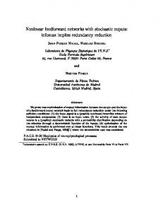
where, at most, two adjacent ’s are positive. For example, the sigmoidal activation function can be approximated over [ 16, 16] via 14 grid points 16, 8, the interval 5, 4, 3, 2, and 1, as shown in Fig. 3(a). Suppose the objective function of (8) is used. Replacing each of the separable nonlinear functions in (17) with the corresponding piecewise linear functions as defined by (22), we obtain an approximating problem to the original SP problem of (17) as follows: Minimize

(20) is the width parameter of , and is the vector where determining the center of From (19) and (20), we can formulate the inverse problem for RBF networks as an SP problem as follows:

Subject to

Minimize

Subject to

.. .

(21)

(22)

LU et al.: INVERTING FEEDFORWARD NEURAL NETWORKS

1277

nonlinear functions involving respectively.

and

as variables in (21),

D. Solving ALP Problems and

and (23) , , are the grid points which are used in where the piecewise linear approximation of the separable nonlinear as variable, and is the number of functions involving grid points. Further, we impose the constraints that for each and no more than two can be positive and only adjacent can be positive. With the exception of the requirement can be positive, on the number and the way in which the the problem of (23) is an linear programming problem. The problem of (23) is called the approximating LP (ALP) problem [1] to the original SP problem of (17). Following the same line as above and using the formulation of (21), we can state the problem of computing INRP for RBF networks as an ALP problem as follows: Minimize

It has been shown that the ALP problems can be solved by use of the simplex method with restricted basis entry rule [35]. For example, the restricted basis entry rule for solving the ALP problem of (23) can be described as follows: is in the basis, then all elements of • If no element of will be allowed to be introduced into the basis, where denotes the set: , , for , , ; and , , 1. is contained in the basis, then only • If one element of the variables adjacent to it are allowed to be introduced into the basis. are contained in the basis, then • If two variables from are allowed to be introduced into the no others from basis. It has been shown that if the objective function is strictly convex and all the constraint functions are convex, the solution obtained from the ALP problems is sufficiently close to the global optimal solution of the original SP problems by choosing a grid of sufficiently short intervals. Unfortunately, the ALP problems of (23) and (24) are nonconvex since the original SP problems have nonlinear equality constraints. Nevertheless, empirical evidence suggests that “even though optimality of the solution can not be claimed with the restricted basis rule, good solutions are produced” [1]. E. Inversion Algorithm Based on SP Techniques

Subject to

and and (24) ’s and two adjacent ’s are where, at most, two adjacent and are the grid points for positive, and respectively, and and are the number of grid points which are used for piecewise linear approximation of

Using the formulations of (17) and (21), we present an SP-based inversion algorithm for inverting MLP’s and RBF networks. The algorithm can be described as follows. Step 1) Set the values of and in (17) or (21). Step 2) Select an objective function. Step 3) Select the number of grid points and the values of the grid points. Step 4) Solve the ALP problems by use of the simplex method with the restricted basis entry rule. If an is found. is the network optimal solution inversion corresponding to the given output, and go to Step 5). Otherwise, go to Step 3) to change the piecewise linear approximation. Step 5) If multiple network inversions are required, go to Step 2) to change the objective function. Otherwise, stop. From optimization’s point of view, the SP-based inversion algorithm is more efficient than the NLP-based inversion algorithm since there are sophisticated computer programs that solve LP problems of very large size. The SP-based inversion algorithm keeps up the same generality as the NLP-based inversion algorithm, except for the restriction that both the objective and constraint functions should be separable. Now let us analyze the complexity of the ALP problems included in the SP-based inversion algorithm. Suppose that output units, and input units, the -layer MLP has

1278

IEEE TRANSACTIONS ON NEURAL NETWORKS, VOL. 10, NO. 6, NOVEMBER 1999

NUMBER

OF

CONSTRAINTS

NUMBER OF CONSTRAINTS

AND

AND

TABLE I VARIABLES IN ALP PROBLEMS

TABLE II VARIABLES IN ALP PROBLEMS

and the number of units in the hidden layer for 1 is Also suppose, for each variable and , and grid points are used. Then the numbers of constraints and variables in the ALP problems formulated for inverting MLP’s are shown in Table I. input, Similarly, suppose that a RBF network has hidden, and output units. Also, suppose, for each variable and , and grid points are used. Thus the number of constraint and variables in the ALP problems formulated for inverting RBF networks are shown in Table II. From Tables I and II, we see that there exists a tradeoff between the accuracy of the approximation of SP problems (i.e., number of grid points) and the complexity of the ALP problems.

F. Relations Between Inversions and Network Parameters In order to sketch out the inverse mapping from the relationships between the given outputs and the corresponding inversions, an ideal inversion algorithm should not only obtain various inversions for a given output as many as possible,

FOR INVERTING

FOR INVERTING

MLPS

RBF NETWORKS

but also provide relationships between the inversions and the network parameters. Almost all existing inversion algorithms such as the iterative inversion algorithm, however, seem to lack abilities to satisfy the latter requirement. In this section, we show that the proposed inversion algorithm for MLP’s as mentioned above makes a step to overcome this deficiency. From (16) we see that once an optimal solution to the NLP problem had been found, we not only get a network inversion but also obtain total net input vectors, i.e., , , Using these total net input vectors, we can establish the relationship between the network inversion and the network parameters. For real-world application problems, the dimension of the input space is usually larger than that of the output space. Consequently, the number of input units in MLP’s is often Consider larger than that of the output units, i.e., three-layer perceptrons, and suppose the inverse mappings formed by the networks are one-to-many mappings. If , all of the possible three-layer perceptrons can be classified into three types, and the parameters of each of them should

LU et al.: INVERTING FEEDFORWARD NEURAL NETWORKS

NETWORK INVERSIONS

1279

OF THE

TABLE III RBF NETWORK

FOR THE

XOR PROBLEM

satisfy one of the following relations: I

rank

II

rank

III

rank

rank rank rank rank rank rank

rank

(25)

rank

(26)

rank

(27)

, , is the weight matrix, where is known total net input vector, and . In the cases of (25) and (26), we see that there exist an for Type infinite number of inversions corresponding to I and II networks. These inversions are determined by the constrained hyper-plane as follows: (28) From (28) we can further compute network inversions by solving the following linear programming problem: Minimize

Subject to (29) , , and are constants, and is variable. where , , For Type III networks, there exists only one network inverConsequently, no inversions can be further find sion for from (28).

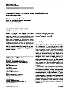
Fig. 1. The mapping from (x1 , x2 ) to y31 formed by the RBF network for the XOR problem.

network in a similar way as presented in [13]. The training data are organized as follows: If the training input is (0, 0) or (1, 1), the corresponding desired output should be zero, and if the training input is (0, 1) or (1, 0), the corresponding desired output should be one. The input–output mapping formed by the trained RBF network is plotted in Fig. 1. 0.7, we state the problem of For a given output computing IMIN’s as the following NLP problem: Minimize Subject to

V. ILLUSTRATIVE EXAMPLES In this section, we present three simple examples to demonstrate the proposed inversion algorithms. For simplicity of illustration, the problems of inverting the RBF network and three-layer MLP which are used to learn the XOR problem are discussed. In the examples except for Example 1, the sigmoidal activation function defined by (18) is used. A. Example 1 In this example, we demonstrate how to invert RBF networks by the NLP-based inversion algorithm. We create a RBF

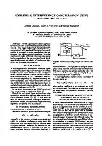
(30) Solving the NLP problem by use of the modified Powell’s method [39], we obtain an IMIN as shown in the first row of Table III. Replacing the objective function of , , , , and (30) with , and solving the corresponding NLP problems, we obtain the related five inversions as shown also in Table III. All the inversions and the corresponding two reference points are illustrated in Fig. 2.

1280

IEEE TRANSACTIONS ON NEURAL NETWORKS, VOL. 10, NO. 6, NOVEMBER 1999

(a)

=

Fig. 2. The network inversions corresponding to the given output y 31 0.7 of the RBF network for the XOR problem. Solid lines denote all the accurate 0.7, squares denote IMIN’s and network inversions associated with y 31 IMAX’s, circles denote reference points, dots denote INRP’s, and dashed lines denote the distance from the reference points to the INRP’s.

=

B. Example 2 A three-layer MLP with two input, two hidden, and one output units is used to learn the XOR problem. The training input and the desired output sets are {(0.01, 0.01), (0.01, 0.99), (0.99, 0.01), (0.99, 0.99)} and {(0.01), (0.99), (0.99), (0.01)}, respectively. The network is trained by the standard backpropagation algorithm [41]. The parameters of the trained XOR network are as follows:

(b) Fig. 3. (a) Piecewise linear approximation of the sigmoidal activation function over the interval [ 16, 16] via 14 grid points 16, 8, 5, 4, 3, 2, and 1. (b) the errors between the original sigmoidal activation function and its approximation as shown in (a).

6

Let us compute IMIN’s and IMAX’s for the given output 0.9 by the SP-based inversion algorithm. Using the formulation of (17) and the parameters of the XOR network mentioned above, we can state the inversion problem as follows: Minimize Subject to

6

0

6 6 6 6 6

corresponding ALP problem. Solving the ALP problem by use of the simplex method with the restricted basis entry as shown in the first rule, we obtain an IMIN and related row of Table IV. Replacing the objective function in the ALP , , and and solving the corresponding problem with ALP problems, we obtain other three network inversions as shown also in Table IV. From Table IV, we see that there exist some errors between the given output and the actual outputs produced by the obtained inversions. The reason for these errors is the piecewise linear approximation of the sigmoidal activation functions. It has been shown that these errors can be reduced by increasing the number of grid points used to approximate the sigmoidal activation functions [34].

C. Example 3 (31) , and and are variables, and the range of where inputs are set to [0.000 001, 0.999 999]. Approximating the sigmoidal activation function over the interval [ 16, 16] via the grid points 16, 8, 5, 4, 3, 2, and 1, as shown in Fig. 3(a), we obtain the

In this example, we demonstrate how to further compute inversions associated with a given by using linear programming techniques. We use the computing results obtained in Example 2. From Table IV, we get the relationship between 0.908 994 and [1.712 502, the given output 2.744 893] Now let us compute the network inversions 0.908 994 by solving the following linear related to

LU et al.: INVERTING FEEDFORWARD NEURAL NETWORKS

1281

TABLE IV NETWORK INVERSIONS AND RELATED TOTAL NET INPUTS OF

COMPUTING RANGES

RELATIONS BETWEEN DIFFERENT



THE

MLP

FOR THE

XOR PROBLEM

TABLE V RELATED NETWORK INVERSIONS

AND

AND THE

TABLE VI CONVERGENCE OF THE ITERATIVE INVERSION ALGORITHM

VI. APPLICATIONS

programming problem: Minimize Subject to

(32) and are variables, and are constants whose where values are shown in Table V. Solving the linear programming problem of (32) under different inequality constraints, we obtain several network inversions as shown in Table V.

OF

NETWORK INVERSIONS

Network inversions have been applied to various problems such as examining and improving the generalization performance of trained networks [26], [28], [12], adaptive control [11] solving inverse kinematics problems for redundant manipulators [18], [16], [7], [33], [2], and speech recognition [38]. In this section we present four examples to illustrate the applications of network inversions obtained by the proposed SP-based inversion algorithm. The first three ones are to illustrate the use of network inversions for examining the generalization performance of trained networks and demonstrate the performance of the proposed inversion algorithm for computing various designated inversions. The last one is presented to show a way of generating boundary training

1282

IEEE TRANSACTIONS ON NEURAL NETWORKS, VOL. 10, NO. 6, NOVEMBER 1999

data for improving the generalization performance of trained networks. A. Generating Test Data Generalization is one of the most important issues in learning of neural networks and refers to a trained network generating reasonable outputs for novel inputs that did not occur during training. In more detail, it can be explained as two different behaviors for dealing with novel inputs, which are commonly known as interpolation and extrapolation, respectively. For existing neural-network models, to achieve a good extrapolation capability is generally much more difficult than to obtain a good interpolation behavior, since a trained network may produce an arbitrary response for a novel input from regions where no training input data have occurred. In practical applications of neural networks, some need networks to have good interpolation capability only, and some require that the networks should both interpolate and extrapolate novel inputs properly. A popular method for examining the generalization performance of trained networks is to measure the performance of the networks on test data that did not presented during training, i.e., the generalization performance of trained networks is judged by the correct recognition rates on the test data. In order to examine generalization performance completely, it is necessary to generate a sufficient number of test data that are distributed in the whole input space. There are two conventional methods for obtaining test data. One is to gather test data from the problem domain, and the other is to generate test data randomly. For most of application problems, it is difficult to obtain a sufficient number of test data by means of the first method because the model of the object to be learned is partially unknown. A difficulty of using random test data is that it is hard to outline the actual decision boundaries formed by the networks especially when the dimension of the input space is high. Our previous work on network inversions has shown that network inversions can be used as a particular kind of test data for detecting generalization errors more completely [28], [31]. In the following three examples, we demonstrate how to generate particular test data by the SP-based inversion algorithm. 1) Fisher’s Iris Classification Problem: In this example, the Fisher’s iris classification problem [8] is treated. It is well known that the iris data set is composed of 150 four-dimensional vectors that measure four features of three varieties of the iris. These data are presented on Fig. 4 by their first and second principal components. The data set is partitioned into a subset with 60 data for training and a subset with 90 data for testing, randomly. A three-layer MLP with four input, three hidden, and two output units are trained by the backpropagation algorithm [41]. First, the trained network is examined by the ordinary 90 test data. The correct recognition rates are 100% for the setosa, 93.3% for the versicolor, and 96.7% for the virginica, respectively. From the above test results, it seems that the network has a nice interpolation performance. However, its extrapolation behavior cannot be judged on these test results

Fig. 4. Fisher’s iris data and the 240 inversions corresponding to the outputs of setosa, which are represented by their two principal components.

Fig. 5. Ten standard printed digit images.

because the test data are distributed in the same areas as the training data. Second, the trained network is examined by network inversions. For simplicity, we consider the IMIN’s and IMAX’s corresponding to the actual outputs of 30 test data for the setosa. By using the SP-based inversion algorithm, 240 inversions are computed, where the sigmoid function is approximated over the interval [ 16, 16] with 14 grid points shown in Fig. 3. The relationships among the 240 inversions and the 150 iris data are also depicted in Fig. 4. From this figure, we can see that the distribution area of the 240 inversions are much wider than that of the training and test data for the setosa. Checking the values of the 240 inversions, we see that, at least, one component of each of the inversions is near zero. Therefore, all the 240 inversions should be judged as unreasonable data according to the physical meaning of the features of the iris. However, the network classifies all the 240 inversions as proper setosa. That is, the network extrapolates all the 240 inversions incorrectly. From this example, we can see that 1) it is difficult to detect extrapolation errors by ordinary test data if their distribution is the same with that of the training data and 2) the network inversions are useful for detecting extrapolation errors. 2) Printed Digits Recognition Problem: We consider the three-layer MLP used for printed digit recognition. Ten standard printed digit images used as training inputs are shown in Fig. 5. Each image corresponds to a vector with each component value varying from zero (white) to one (black) determined by the gray level in the corresponding pixel. Four output units are used to represent ten classes of outputs according to the binary coding method. A three-layer MLP with 35 input units, 12 hidden units, and four output units is used to learn this pattern recognition task.

LU et al.: INVERTING FEEDFORWARD NEURAL NETWORKS

Fig. 6. Random test input images for digit “0.” All them are recognized as the proper digit “0,” except one marked by open gray box. The images from left to right are numbered from 1 to 10.

The training data set consists of ten standard training patterns and 540 noised training patterns. The noised training inputs are generated by performing logic XOR operation between the ten standard training inputs and the 540 noise patterns. The noise patterns for generating noised training inputs are created by randomly putting three black pixels in the 35 white pixels according to a uniform distribution. In the following, the noise pattern which is generated by randomly 35) blank pixels in the 35 white pixels putting (1 is called the -random-dots pattern. According to combination theory, the total number of different noise patterns (binary value) is 2 Random Test Data: In order to compare the test data obtained by the SP-based inversion algorithm with the test data generated randomly, we first discuss the characteristics of the random test data. For simplicity of description, we consider the random test input images for digit “0.” Ten random test input images are generated by doing the logical XOR operation between the standard training inputs of “0” and ten fiverandom-dots patterns. Fig. 6 illustrates these random test input images. Presenting these random test input images to the trained network and checking the corresponding outputs, we see that all the ten random test input images, except one image, are classified as digit “0” by the network. Comparing the standard digit images in Fig. 5 with the random test images in Fig. 6, we can see that the network produces several generalization errors. For example, the second random test input image in Fig. 6 is recognized as the digit “0” by the network. However, one may answer that it is not digit “0” from the viewpoint of human recognition. From this example, we see that the network may assign some poor novel input images to one of the known digits. For some practical applications, for instance fault diagnosis systems [21], [23], it is necessary to remove this kind of generalization errors since fault inputs may be classified as the normal states or normal inputs may be classified as the fault states by the network if this kind of incorrect generalizations exist. To remove this kind of generalization errors completely, we should outline the actual inverse images of given outputs. However, it is very difficult to achieve this objective by using random test data, especially for high-dimensional input space. The reason is that to generate all random test inputs which will give rise to a given output random test input images, where is the needs to check number of input units and is the number of values which can be taken from each pixel. For example, we need to examine 2 test input images for the printed digit recognition problem even if considering only binary value patterns. Network Inversions as Test Data: Selecting the objective and solving the corresponding ALP functions as problems, we obtain various network inversions as illustrated

1283

Fig. 7. The five IMIN’s and five IMAX’s corresponding to the actual output of standard digit “0.” The ten images from left to right are arranged as the 1)th image (in odd column) is the IMIN obtained by following: the (2i minimize xi , and the (2i)th image (in even column) is the IMAX obtained by maximize xi for i 6, , 10. The pixels to be optimized as the objective function are marked by small open gray boxes. If the given level in a pixel is white (black), the value of the related component is 0 (1). This notation will be also used in Figs. 8–14.

0 = 111

(a)

(b) Fig. 8. The inversions (upper ten images) obtained by minimizing the sum of the values of the pixels in the upper center area, i.e., (x7 + x8 + x9 + x12 + x13 + x14 ), and the inversions (lower ten images) obtained by maximizing the same objective function.

Fig. 9. The inversions (upper ten images) obtained by minimizing the sum of all the pixels, i.e., 6i35 =1 xi , and the inversions (lower ten images) obtained by maximizing the same objective function.

in Figs. 7–9. The central processing unit (CPU) time for computing each of these inversions is about 8 s at a SUN Ultra workstation. Here, the sigmoidal activation functions is approximated over the interval [ 16, 16] with 26 grid points. for Choosing the objective function as we obtain five IMIN’s and five IMAX’s for the actual output of the standard digit “0.” Fig. 7 shows five IMIN’s and five IMAX’s. From these inversions, we know that the actual range 6, 10) component of the inverse image of the th (for is between zero and one. Presenting the ten inversions to the network and checking the corresponding outputs, we see that all the inversions are recognized as the standard digit “0” by the network. Clearly, these generalizations are incorrect from the viewpoint of human decision. Furthermore, selecting the objective functions as and and we obtain 40 inversions as illustrated in Figs. 8 and 9 by using the SPbased inversion algorithm. Here, the given outputs are set to the actual outputs of the ten standard digits shown in Fig. 5. Looking at the 40 images in Figs. 8 and 9, we may indistinctly recognize a few images among them as the digit “7” and “9” in a usual way. Checking the actual outputs of the inversions, however, we see that all the inversions are recognized as the standard digits by the network.

1284

IEEE TRANSACTIONS ON NEURAL NETWORKS, VOL. 10, NO. 6, NOVEMBER 1999

Fig. 10. Ten random inversions for digit “0” obtained by the iterative inversion algorithm.

Fig. 11.

Digits that were segmented from handwritten ZIP codes.

Fig. 14. Thirty particular images derived from the 300 inversions. All these images are also recognized as proper handwritten digits by the network.

Fig. 12. Illustrations of 15 different objective functions which are defined as the sums of the elements in the shadow areas, for example, the upper-left 16 frame represents the objective function, 615 i=0 6j =1 x16i+j : The 15 frames from left to right and from top to bottom are numbered from 1 to 15.

Fig. 13. Inversions corresponding to the actual outputs of the handwritten digits “0”–“9,” respectively. These inversions are obtained by using the objective function of minimizing the sum of the pixels located in the shadow area of the first frame in Fig. 12.

In order to compare the inversions obtained by the SPbased inversion algorithm with these obtained by the iterative inversion algorithm, ten random inversions for the actual outputs of the digit “0” are also computed by the iterative inversion algorithm. The starting points are generated randomly according to a uniform distribution. The average CPU time for computing each of the inversions is about 0.02 s. Fig. 10 illustrates the ten random inversions. Although the iterative inversion algorithm is much faster than the SP-based inversion algorithm, it is hard for the user to roughly outline the actual inverse images of given outputs from the random inversions. From the simulation results mentioned above, we see that the proposed inversion method for generating test data possesses the following two features in comparison with the method of generating test data randomly and the iterative inversion algorithm. 1) Various designated network inversions corresponding to a given output can be obtained efficiently

by the proposed inversion algorithm. 2) These inversions are useful for roughly outlining the actual inverse image of a given output, and therefore the extrapolation behavior of trained networks can be examined more systematically. 3) Handwritten ZIP Code Recognition Problem: We deal with the handwritten ZIP code recognition problem [25], one of typical applications of feedforward neural networks to real-world pattern recognition problems. The aims to solve this problem are to show the effectiveness of the SP-based inversion algorithm for inverting large-scale neural networks and to demonstrate the usefulness of network inversions for detecting particular extrapolation errors. The original training set and test set (TEST1) for the handwritten ZIP code recognition problem consist of 7291 and 2007 data, respectively. Fig. 11 shows ten handwritten numerals that were segmented from the handwritten zip codes. The image for each handwritten ZIP code data contains 16 pixel rows by 16 pixel columns, for a total 256 pixels. Since it is hard to learn the whole 7291 training data by using a conventional threelayer MLP, we randomly select 500 training data from the original training set as a reduced training set. The remaining 6791 training data are considered as a new test set (TEST2). The desired outputs are represented by the binary coding method. A three-layer MLP with 256 input units, 30 hidden units, and four output units is trained on the reduced training set by the backpropagation algorithm [41]. After training of the network, its generalization performance is examined on the ordinary test data. The correct recognition rates on TEST1 and TEST2 are 78.1 and 82.9%, respectively. Although the total number of the test data is much more than that of the training data, the generalization performance of the network cannot be judged only on the above correct recognition rates because the test data are not distributed in the whole input space and many generalization errors, especially

LU et al.: INVERTING FEEDFORWARD NEURAL NETWORKS

(a)

1285

(b)

Fig. 15. Two-class classification problem. (a) The desired input-output mapping. (b) The initial 40 random training inputs, which are represented by small open boxes and filled triangles. The desired outputs for the open boxes and filled triangles should be zero and one, respectively. The big triangle (dashed) denotes the desired decision boundary associated with output 0.8. This notation will be used in Figs. 16–19.

extrapolation errors, may not be detected. In the following, we demonstrate how to detect particular extrapolation errors in a more systematic way by using network inversions. Selecting the objective functions as minimizing and maximizing the sum of the pixels located in the shadow areas depicted in Fig. 12 and solving the corresponding ALP problems, we obtain 300 network inversions for the actual outputs of the handwritten digits “0”–“9” shown in Fig. 11. Here, the sigmoidal activation function is approximated over the interval [ 16, 16] with 14 grid points shown in Fig. 3. The average CPU time for computing each of these inversions is about 14 min. Fig. 13 illustrates 20 inversions that are obtained by minimizing the sum of 60 pixels located in the shadow area of the first frame in Fig. 12. The frames from left to right and from top to bottom in Fig. 13 are the inversions for the actual outputs of the handwritten digits “0”–“9,” respectively. Examining each image of the 300 inversions, we see that all of them are poor images and no one can be recognized as the handwritten digits from the viewpoint of human decision. However, all of the 300 inversions are recognized as proper handwritten digits by the network. For example, the inversions from left to right and from top to bottom in Fig. 13 are recognized as proper handwritten digits “0”–“9” by the network, respectively. Clearly, these generalizations are incorrect. Fig. 14 illustrates 30 particular images which are derived from the 300 inversions with reference to the similar inversions. For example, the particular image in the first frame of Fig. 14 is derived from the inversion in the first frame of Fig. 13. Presenting the 30 particular images to the network and checking the corresponding actual outputs, we find that all the 30 particular images are also recognized as the proper handwritten digits by the network. For example, the 1st image in Figs. 14 is recognized as proper handwritten “0” by the network. If we examine the generalization performance of the network by using the ordinary test data, we may never think that the network will produce so poor generalization.

In most of practical applications, we need to detect extrapolation errors more completely. Therefore, various network inversions for different given outputs should be obtained. From this example, we can see that the proposed SP-based inversion algorithm may provide us with an efficient tool for dealing with this problem. B. Generating Boundary Training Data It has been observed that using training data located at the boundaries of decision regions gives better performance than using training data selected randomly [37], [12]. The training data located at the boundaries of the decision regions are called the boundary training data. In this example, we demonstrate how to generate the boundary training data by inverting trained networks with our inversion method and illustrate the effectiveness of the boundary training data for improving the generalization performance of trained networks. Following the similar way presented in [12], we use network inversions as the boundary training data and retrain the network to improve its generalization performance. The network inversions which produce correct generalization are used as “positive” retraining data, and the others are used as “negative” retraining data, i.e., counter-samples. The purpose of the “positive” retraining data is to consolidate the domain of the input space on which the network generalizes correctly. On the contrary, the “negative” retraining data are to narrow the range of each input variable to reduce the domain of the input space on which the network produces incorrect generalization. For visualization of the decision boundary formed by the network, a simple two-class pattern recognition problem is treated. The problem is to classify two-dimensional inputs into two classes. The desired input-output mapping is shown in Fig. 15(a). For the inputs inside a triangle region as shown in Fig. 15(b), the network should give rise to output 0.99, and otherwise the output should be 0.01. The initial 40 training data illustrated in Fig. 15(b) are generated randomly according

1286

IEEE TRANSACTIONS ON NEURAL NETWORKS, VOL. 10, NO. 6, NOVEMBER 1999

(a)

(b)

Fig. 16. (a) The input–output mapping formed by the network which is trained on the 40 random training data. (b) The inversions (small open circles) and the actual decision boundary (close curve) associated with output 0.8.

(a)

(b)

(c)

(d)

Fig. 17. The process of improving the generalization performance of the network by retraining the network with the network inversions as the boundary training data. (a), (c), (e), and (g) represent the retraining inputs for the first, the second, the third, and fourth retraining, respectively. (b), (d), (f), and (h) represent the inversions (small open circles) obtained from the corresponding trained networks and the actual decision boundaries formed by the networks after the first, the second, the third, and the fourth retraining, respectively.

LU et al.: INVERTING FEEDFORWARD NEURAL NETWORKS

1287

(e)

(f)

(g)

(h)

Fig. 17. (Continued.) The process of improving the generalization performance of the network by retraining the network with the network inversions as the boundary training data. (a), (c), (e), and (g) represent the retraining inputs for the first, the second, the third, and fourth retraining, respectively. (b), (d), (f), and (h) represent the inversions (small open circles) obtained from the corresponding trained networks and the actual decision boundaries formed by the networks after the first, the second, the third, and the fourth retraining, respectively.

(a)

(b)

Fig. 18. (a) The input–output mapping formed by the network after the fourth retraining with 40 random and 56 boundary training data. (b) The corresponding actual decision boundary.

1288

IEEE TRANSACTIONS ON NEURAL NETWORKS, VOL. 10, NO. 6, NOVEMBER 1999

(a)

(b)

(c) Fig. 19. (a) 200 random training inputs. (b) The input–output mapping formed by the network which is trained on 200 random training data. (c) The corresponding actual decision boundary.

to a uniform distribution in the two-dimensional input space. A three-layer perceptron with two input, ten hidden, and one output units is used to learn this problem. Here, the decision boundary is defined as a curve in the input space, on which the corresponding outputs are about 0.8. After the network is trained with the 40 random training data, we generate boundary training data, i.e., network inversions, by inverting the trained network, and improve the generalization performance by retraining the network with the boundary training data according to the following procedure. and respecStep 1: Compute two IMIN’s, i.e., and respectively, tively, and two IMAX’s, i.e., 0.8. associated with the given output Step 2: Generate ten reference points randomly and compute the corresponding ten INRP’s associated with the given 0.8. output Step 3: Examine the generalization performance of the trained network by using the 14 inversions (i.e., two IMIN’s, two IMAX’s, and ten INRP’s) and their corresponding outputs. Step 4: If the decision boundary outlined by the inversions is satisfactory to compare with the desired decision boundary,

then stop the procedure. Otherwise, do the following steps. Step 5: Adding the test results to the training set, we obtain an extended retraining set. The obtained inversions are classified into positive and negative data according to their desired outputs. Step 6: Retrain the network on the extended retraining set and go back to Step 1). In the above procedure, the reason for using IMIN’s, IMAX’s, and INRP’s as the boundary training data is that IMIN’s and IMAX’s can give rough estimates of the range of the decision boundary and INRP’s can outline the decision boundary in more detail. All of the network inversions are obtained by solving the corresponding ALP problems. The method described here is general and can be applied to -class 2) pattern recognition problems. ( Repeating the above procedure four times, the generalization performance of the network is improved significantly. The process of improvement is shown in Figs. 16–18. The final result after the fourth retraining is shown in Fig. 18. Comparing Fig. 18 with Fig 16, we see that much better generalization performance is obtained. In order to compare the effectiveness

LU et al.: INVERTING FEEDFORWARD NEURAL NETWORKS

of the boundary training data with that of random training data, the network is trained on 200 random training data. Fig. 19 shows the corresponding training inputs, the actual input–output mapping, and the decision boundary formed by the trained network. Comparing Fig. 18 with Fig. 19, we see that the boundary training data obtained by our inversion algorithms is much superior to the random training data in the generalization performance of the trained networks.

1289

[5] [6] [7] [8] [9] [10]

VII. CONCLUSIONS We have formulated the inverse problems for feedforward neural networks as constrained optimization problems. We have shown that the problems of inverting MLP’s and RBF networks can be formulated as separable programming problems, which can be solved by a modified simplex method, a well-developed and efficient method for solving linear programming problems. As a result, various network inversions of large-scale MLP’s and RBF networks can be obtained efficiently. We have presented three inversion algorithms based on NLP, SP, and LP techniques. Using the proposed inversion algorithms, we can obtain various designated network inversions for a given output. We have shown that the proposed method has the following three features: 1) The user can explicitly express various functional and (or) side constraints on network inversions and easily impose them on the corresponding constrained optimization problems. 2) Various designated network inversions for a given output can be obtained by setting different objective and constraint functions. 3) Once the network inversions for MLP’s have been found, the relationship between the network inversions and the network parameters is also brought to light. We have compared the proposed inversion method with the iterative inversion algorithm and analyzed the limitations of the iterative inversion algorithm. We have also demonstrated the applications of the network inversions obtained by the SP-based inversion algorithm to examining and improving the generalization performance of trained networks. The simulation results show that the network inversions are useful for detecting generalization errors and improving the generalization performance of trained networks. ACKNOWLEDGMENT The authors are grateful to Prof. T. Tezuka of Kyoto University for his valuable suggestions and discussions on this research and S. Murakami for his help in computer simulations. The authors also would like to thank the anonymous referees for improvements to the article, as suggested by their comments.

[11] [12] [13] [14] [15] [16] [17] [18]

[19] [20] [21] [22] [23] [24] [25]

[26] [27]

[28] [29] [30]

REFERENCES [1] M. B. Bazaraa, H. D. Sherali and C. W. Shetty, Nonlinear Programming Theory and Algorithms, 2nd ed. New York: Wiley, 1993. [2] L. Behera, M. Gopal, and S. Chaudhury, “On adaptive trajectory tracking of a robot manipulators using inversion of its neural emulator,” IEEE Trans. Neural Networks, vol. 7, pp. 1401–1414, 1996. [3] C. W. Bishop, Neural Networks for Pattern Recognition. Oxford, U.K.: Oxford Univ. Press, 1995. [4] C. W. Bishop and C. Legleye, “Estimating conditional probability densities for periodic variables,” in Advances in Neural Information

[31] [32] [33]

Processing Systems, G. Tesauro, D. S. Touretzky, and T. K. Leen, Eds., vol. 7. Cambridge, MA: MIT Press, 1995, pp. 641–648. V. Chv´atal, Linear Programming San Francisco, CA: W. H. Freeman, 1983. D. Colton and R. Kress, Inverse Acoustic and Electromagnetic Scattering Theory. Berlin, Germany: Springer-Verlag, 1992. D. E. Demers, “Learning to invert many-to-one mapping,” Ph.D. dissertation, Univ. California, San Diego, 1992. R. A. Fisher, “The use of multiple measurements in taxonomic problems,” Ann. Eugenics, vol. 7, pt. 2, pp. 179–188, 1936. C. L. Giles and T. Maxwell, “Learning, invariance, and generalization in high-order neural networks,” Appl. Opt., vol. 26, pp. 4972–4978, 1987. G. M. L. Gladwell, Inverse Problems in Vibration. Dordrecht, The Netherlands: Kluwer, 1986. D. A. Hoskins, J. N. Hwang, and J. Vagners, “Iterative inversion of neural networks and its application to adaptive control,” IEEE Trans. Neural Networks, vol. 3, pp. 292–301, 1992. J. N. Hwang, J. J. Choi, S. Oh, and R. J. Mark, II, “Query based learning applied to partially trained multilayer perceptrons,” IEEE Trans. Neural Networks, vol. 2, pp. 131–136, 1991. S. Haykin, Neural Networks. New York: Macmillan, 1994. Y. Iiguni, H. Sakai, and H. Tokumaru, “A real time learning algorithm for a multilayered neural network based on extended Kalman filter,” IEEE Trans. Signal Processing, vol. 40, 1992. R. A. Jacobs, M. I. Jordan, M. I. Nowlan, and G. E. Hinton, “Adaptive mixtures of local experts,” Neural Comput., vol. 3, pp. 79–87, 1991. M. I. Jordan and D. E. Rumelhart, “Forward models: supervised learning with a distal teacher,” Cognitive Sci., vol. 16, pp. 307–354, 1992. M. I. Jordan and R. A. Jacobs, “Hierarchical mixtures of experts and the EM algorithm,” Neural Comput., vol. 6, pp. 181–214, 1994. M. Kawato, “Computational schemes and neural network models for formation and control of multijoint arm trajectory,” in Neural Networks for Control, W. T. Miller, R. S. Sutton, and P. J. Werbos Eds. Cambridge, MA: MIT Press, 1990, pp. 197–228. J. Kindermann and A. Linden, “Inversion of neural networks by gradient descent,” Parallel Computing, vol. 14, pp. 277–286, 1990. A. Kirsch and R. Kress, “A numerical method for an inverse scattering problem,” in Inverse and Ill-posed Problems, H. W. Engl and C. W. Groetsch, Eds. Boston: Academic, 1987. M. A. Kramer and J. A. Leonard, “Diagnosis using backpropagation neural networks: Analysis and criticism,” Computers Chem. Eng., vol. 14, pp. 1323–1338, 1990. M. Kuperstein, “neural model of adaptive hand-eye coordination for single postures,” Science, vol. 239, pp. 1308–1311, 1988. J. A. Leonard and M. A. Kramer, “Radial basis function networks for classifying process faults,” IEEE Contr. Syst. Mag., vol. 11, pp. 31–38, 1991. S. Lee and R. M. Kil, “Inverse mapping of continuous functions using local and global information,” IEEE Trans. Neural Networks, vol. 5, pp 409–423, 1994. Y. Le Cun, Y. B. Boser, J. S. Denker, D. Henderson, R. E. Howard, W. Hubbard, and L. D. Jackel, “Backpropagation applied to handwritten ZIP code recognition,” Neural Computation, vol. 1, no. 4, pp. 541–551, 1989. A. Linden, and J. Kindermann, “Inversion of multilayer nets,” in Proc. Int. Joint Conf. Neural Networks, Washington, D.C., 1989, pp. II425–II430. A. Linden, “Iterative inversion of neural networks and its applications,” in Handbook of Neural Computation, M. Fiesler and R. Beale Eds. Oxford, U.K.: Inst. Phys. Publishing and Oxford Univ. Press, 1997, pp. B521–B527. B. L. Lu, H. Kita, and Y. Nishikawa, “Examining generalization by network inversions,” in Proc. 1991 Annu. Conf. Japanese Neural Network Soc., Tokyo, Japan, 1991, pp. 27–28. , “A new method for inverting nonlinear multilayer feedforward networks,” in Proc. IEEE Int. Conf. Ind. Electron. Contr. Instrumentation, Kobe, Japan, Oct. 28–Nov. 1, 1991, pp. 1349–1354. B. L. Lu, Y. Bai, H. Kita, and Y. Nishikawa, “An efficient multilayer quadratic perceptron for pattern classification and function approximation,” in Proc. Int. Joint Conf. Neural Networks, Nagoya, Japan, Oct. 25–29, 1993, pp. 1385–1388. B. L. Lu, H. Kita, and Y. Nishikawa, “Inversion of feedforward neural networks by a separable programming,” in Proc. World Congr. Neural Networks, Portland, OR, July 11–15, 1993, pp. IV415–IV420. B. L. Lu, “Architectures, learning and inversion algorithms for multilayer neural networks,” Ph.D. dissertation, Dept. Elect. Eng., Kyoto Univ., Japan, 1994. B. L. Lu and K. Ito, “Regularization of inverse kinematics for redundant manipulators using neural network inversions,” in Proc. IEEE Int.

1290

[34]

[35] [36] [37] [38] [39] [40] [41]

[42] [43] [44]

IEEE TRANSACTIONS ON NEURAL NETWORKS, VOL. 10, NO. 6, NOVEMBER 1999

Conf. Neural Networks, Perth, Australia, Nov. 27–Dec. 1, 1995, pp. 2726–2731. , “Transformation of nonlinear programming problems into separable ones by multilayer neural networks,” in Mathematics of Neural Networks: Models, Algorithms, and Applications, S. W. Ellacott, J. C. Mason, and I. J. Anderson, Eds. Boston, MA: Kluwer, 1997, pp. 235–239. C. E. Miller, “The simplex method for local separable programming,” in Recent Advances in Mathematical Programming, R. L. Graves and P. Wolfe, Eds. New York: McGraw-Hill, 1963, pp. 89–100. W. T. Miller, “Sensor-based control of robotic manipulators using a general learning algorithm,” IEEE J. Robot. Automat., vol. 3, pp. 157–165, 1987. K. G. Mehrotra, C. K. Mohan, and S. Ranka, “Bounds on the number of samples needed for neural learning,” IEEE Trans. Neural Networks, vol. 2, pp. 548–558, 1991. S. Moon and J. N. Hwang, “Robust speech recognition based on joint model and feature space optimization of hidden Markov models,” IEEE Trans. Neural Networks, vol. 8, pp. 194–204, 1997. M. J. D. Powell, “A fast algorithm for nonlinearly constrained optimization calculations,” in Lecture Notes in Mathematics 630, G. A. Watson, Ed. Berlin: Springer-Verlag, 1978. S. S. Rao, Engineering Optimization: Theory and Practice, 3rd ed. New York: Wiley, 1996. D. E. Rumelhart, G. E. Hinton, and R. J. Williams, “Learning internal representations by error propagation,” in Parallel Distributed Processing: Exploration in the Microstructure of Cognition, vol. 1, D. E. Rumelhart, J. L. McClelland, and PDP Research Group, Eds. Cambridge, MA: MIT Press, 1986, pp. 318–362. R. S. Scalero and N. Tepedelenlioglu, “A fast new algorithm for training feedforward neural networks,” IEEE Trans. Signal Processing, vol. 40, 1992. R. Shamir, “The efficiency of the simplex method: A survey,” Management Sci., vol. 33, pp. 301–334, 1987. R. J. Williams, “Inverting a connectionist network mapping by backpropagation of error,” in Proc. 8th Annu. Conf. Cognitive Sci. Soc.. Hillsdale, NJ: Lawrence Erlbaum, 1986, pp. 859–865.

Bao-Liang Lu (M’94) was born in Qingdao, China, on November 22, 1960. He received the B.S. degree in instrument and control engineering from Qingdao Institute of Chemical Technology, Qingdao, China, in 1982, the M.S. degree in computer science and engineering from Northwestern Polytechnical University, Xi’an, China, in 1989, and the Ph.D degree in electrical engineering from Kyoto University, Kyoto, Japan, in 1994. From 1982 to 1986, he was with the Qingdao Institute of Chemical Technology. From April 1994 to March 1999, he was a Frontier Researcher at the Bio-Mimetic Control Research Center, the Institute of Physical and Chemical Research (RIKEN), Japan. Currently he is a Staff Scientist at the Brain Science Institute, RIKEN. His research interests include neural networks, brain-like computers, pattern recognition, mathematical programming, and robotics. Dr. Lu is a member of Japanese Neural Network Society, the Institute of Electronics, Information and Communication Engineers of Japan, and the Robotics Society of Japan.

Hajime Kita received the B.E, M.E., and Ph.D. degrees in electrical engineering from Kyoto University, in 1982, 1984, and 1991, respectively. From 1987 to 1997, he worked as an Instructor at the Department of Electrical Engineering, Kyoto University. Since 1997, he has been an Associate Professor at the Department of Computational Intelligence and Systems Science, Tokyo Institute of Technology. His research interests are evolutionary computation, neural networks, and socio-economic analysis of energy systems. Dr. Kita is a member of the Institute of Electrical Engineers of Japan, the Institute of Electronics, Information and Communication Engineers of Japan, the Institute of Systems, Control and Information Engineering of Japan, Japanese Neural Network Society, Japan Society of Energy and Resources, the Operations Research Society of Japan, and the Society of Instrument and Control Engineers of Japan.

Yoshikazu Nishikawa was born in OhmiHachiman, Japan, on March 18, 1933. He received the B.S, M.S., and the Doctor of Engineering (Ph.D) degrees, all from Kyoto University, Japan, in 1955, 1957, and 1962, respectively. In 1960, he joined the Department of Electrical Engineering, Faculty of Engineering, Kyoto University. Since 1972, he has been Professor of the Laboratory of Instrument and Control Engineering, Faculty of Engineering, and also the Laboratory of Complex Systems Science and Engineering, Graduate School of Engineering, Kyoto University. From 1993 to 1996, he was Dean of the Faculty of Engineering and the Graduate School of Engineering, and also Vice President of the University. Since April, 1996, after retirement from Kyoto University, he has been Dean and Professor of the Faculty of Information Sciences, Osaka Institute of Technology, Japan. His research interest includes systems planning, systems optimization, systems control, nonlinear systems analysis and synthesis, especially those of complex systems. He is currently working on bioinformatics including neural networks, evolutionary algorithms and artificial life, and also autonomous decentralized and/or emergent function generation approaches to complex systems planning, design, and operation. Dr. Nishikawa is a member of the Science Council of Japan and many other organizations on Science and Engineering.