in this volume, as well as in several good books, notably Vidyasagar (1997).) The VC dimension is geared towards binary classification. It is possible.
VC Dimension of Neural Networks Eduardo D. Sontag Department of Mathematics, Rutgers, The State University of New Jersey Abstract. This paper presents a brief introduction to Vapnik-Chervonenkis (VC) dimension, a quantity which characterizes the difficulty of distribution-independent learning. The paper establishes various elementary results, and discusses how to estimate the VC dimension in several examples of interest in neural network theory.
1
Introduction
In this expository paper, we present a brief introduction to the subject of computing and estimating the VC dimension of neural network architectures. We provide precise definitions and prove several basic results, discussing also how one estimates VC dimension in several examples of interest in neural network theory. We do not address the learning and estimation-theoretic applications of VC dimension. (Roughly, the VC dimension is a number which helps to quantify the difficulty when learning from examples. The sample complexity, that is, the number of “learning instances” that one must be exposed to, in order to be reasonably certain to derive accurate predictions from data, is proportional to this number. This relationship can be made mathematically precise using the formalism of computational learning theory and uniform convergence theorems for empirical probabilities, and it is covered in other papers in this volume, as well as in several good books, notably Vidyasagar (1997).) The VC dimension is geared towards binary classification. It is possible to generalize the notion of VC dimension in several ways, to deal with the problem of “learning” (approximating from data) real-valued functions. This leads to pseudodimension (Haussler 1992, Vidyasagar 1997), “fat-shattering dimension” (Anthony and Bartlett n.d.), and several other notions. Reasons of space preclude covering such topics in this paper; however, many of the tools developed here are also central to the study of these generalizations.
2
Concepts and VC Dimension
As a starting point for introducing the necessary concepts, we assume given a set U, to be called the input space. Typically, U will be a subset of Rm , for some m; we think of inputs as vectors whose coordinates may represent “features” to be used for classification purposes. Also given is a concept class C, which consists of a family of subsets of U. Some examples of input spaces and concept classes are as follows:
2
1. 2. 3. 4.
Eduardo D. Sontag
U = R, C = infinite open intervals, or the empty set; U = R, C = R, ∅, one open interval, or two disjoint infinite open intervals; U = R2 , C = open half-spaces; and U = R2 , C = all convex sets.
Definition 1 A finite subset S ⊆ U is shattered by C if (∀ S+ ⊆ S) (∃ C ∈ C) S+ = S
\
C.
(1)
For the above examples, we have that one may shatter, respectively: 1. 2. 3. 4.
every 2-element set, no 3-element set; every 3-element set, no 4-element set; every noncollinear 3-element set, no 4-element set; and any finite subset of unit circle.
The first two of these are quite clear. To see that no 4-element set S ⊆ R2 can be shattered when C = all open half-spaces, we can argue as follows (see Fig. 1). If some three points of S lie on a line, then S cannot be shattered, because it is impossible to find a half-space which covers only the midpoint. Similarly if one of the points lies in the convex hull of the remaining three points. On the other hand, if no three points lie on a line, then S determines the corners of a quadrilateral, and a set S+ which consists of one pair of opposing corners cannot be the intersection of S and a half-plane. To see that any finite subset of the unit circle can be shattered, in the last example, we may pick any such subset S, and any subset S+ ⊆ S, and take the convex hull of S+ as the desired element of C (this set is the region inside a polygon whose vertices are the points in S+ ). e �A � A
e ��
�� � u � e ��
e
A � A � u A � e PP A PP PP A PPAe
uX X XX X Xe
e hh h h
hhhhu
Fig. 1. Four points cannot be shattered by half-spaces
Definition 2 The Vapnik-Chervonenkis (VC) dimension of C is: vcd (C) := sup { card S | S shattered by C}
(2)
VC Dimension of Neural Networks
3
In the above examples, one obtains, respectively: 2, 3, 3, ∞. (Observe that, in the third example, sets of three points that are in a straight line cannot be shattered. Nonetheless, the VC dimension is 3 because some 3-element set can be shattered; as a matter of fact, it turns out in this particular example that “almost any” 3-element set can be shattered, but this is not required in the definition.)
Equivalently, with Functions The concept-based definition of VC dimension just given originates in combinatorics and computer science. It is useful to provide an equivalent formulation in terms of functions, which is the way in which the subject arises in statistical estimation. Now, instead of C, we assume given a function class F, consisting of a set of binary functions U → {0, 1}. To each f ∈ F we may associate the set Cf = {u ∈ U | f (u) = 1}
(3)
and thus to F we associate a concept class CF := {Cf , f ∈ F } .
(4)
vcd (F) := vcd (CF ) .
(5)
We define:
Conversely, to any concept class C we may associate a function class F in such a way that C = CF (just take characteristic functions of subsets). We use the two formalisms interchangeably, depending on which is more convenient for any given proof. Actually, in practice one is often interested in classifiers which arise from neural networks and other devices which produce real-valued outputs, and one makes the convention that positive outputs are interpreted as “1” and negative outputs as “0” for purposes of binary classification. Formally, we are now given a set of real-valued functions F, and define, then: vcd (F) := vcd ({H ◦ f, f ∈ F }) ,
(6)
where H(x) is the “Heaviside” function which equals 1 if x > 0 and equals 0 if x ≤ 0. (In other words, a “concept” is a set where some possible f ∈ F is positive.) We also write sign x = H(x). In this language, saying that a subset S = {u1 , . . . , un } ⊆ U is shattered means that, for any possible binary assignment ε = (ε1 , . . . , εn ) ∈ {0, 1}n , there must exist some function f = fε ∈ F which has precisely these signs, i.e., H(f (ui )) = εi .
4
Eduardo D. Sontag
Parametrized Classes of Functions The class F is more often than not specified by means of neural network architectures with tunable weights, or some other parametric description (splines with nodes and values to be determined, Fourier series with a fixed number of terms but adjustable frequencies and coefficients, etc). In general, we may suppose given a function β : W × U → R. (7) Typically, W = Rρ , where ρ is called the number of weights or parameters, and w = (w1 , . . . , wρ ) ∈ W is a weight or parameter vector . For each choice of parameters, we obtain a function: Fβ := { β(w, ·) | w ∈ W}
(8)
vcd (β) := vcd (Fβ ) .
(9)
and we define We can express the first three examples given earlier in this language, as follows: � 1. the map β : R2 × R → R given by β (a, b), u := a + bu leads to the concept class C which consists of all open infinite � intervals (and ∅); 2. the map β : R3 × R → R given by β (a, b, c), u := a + bu + cu2 leads to the second example (R, ∅, one open interval, or two disjoint infinite open intervals); and � 3. the map β : R3 × R2 → R given by β (a, b, c), (u, v) := a + bu + cv leads to the third one (half-spaces). Observe that in all these examples, the parametric description β is linear in the parameters a, b, and c, and the VC dimension coincides with the respective number of parameters. This is not a coincidence, as we see next.
3
Special Case: Linear Parameterizations
Linearly parametrized classes constitute vector spaces; their dimension is the number of independent parameters. Elementary linear algebra gives that the linear dimension of a vector space of functions F is finite, and equal to n, if and only if there is a set of n functions {f1 , . . . , fn } ⊆ F, and there are some n points u1 , . . . , un , so that the following matrix:
A =
u1 u2 .. .
f1 f1 (u1 ) f1 (u2 ) .. .
··· ··· ··· .. .
fn fn (u1 ) fn (u2 ) .. .
un
f1 (un ) f2 (un ) · · ·
fn (un )
f2 f2 (u1 ) f2 (u2 ) .. .
(10)
has rank n, and any n + 1 by n + 1 matrix of this type is singular. The following general fact is very useful for linear classes:
VC Dimension of Neural Networks
5
Theorem 1. If F is a vector subspace of RU , then vcd F = dim F. Proof. Saying that a subset S = {u1 , . . . , un } ⊆ U is shattered by F is the same as saying that there exists some set of 2n functions, let us say f1 , . . . f2n , for which the columns of the array fj (ui ) assume all possible 2n sign vectors, that is, we have a sign pattern as follows (after if necessary rearranging the fi ’s): f1 f2 f3 · · · f2n u1 − − − ··· + − − − ··· + u2 (11) B = .. .. .. .. .. . . . . ··· . un−1 un
− −
− +
+ −
··· ···
+ +
(using “−” to mean entries ≤ 0). Pick any n, and suppose that the VC dimension of F (which could be infinite) is ≥ n. By definition, there is some subset S = {u1 , . . . , un } ⊆ U which is shattered. We claim that this matrix B has rank n (the number of rows). Indeed, if this is not the case, then the rows are linearly independent, i.e., there is some vector ν 6= 0 so that νB = 0. Assume that there is such a vector, and consider the vector of signs of ν, say (+, +, −, +, . . . +). Now pick that column fi of B which has exactly these signs. The inner product ν · fi is obviously positive (sum of nonnegative terms, at least one nonzero), contradicting νB = 0. Since rank B = n, there are n linearly independent columns, let us say fi1 , . . . , fin . These give rise to a submatrix A as in (10), so dim F ≥ n. As this holds for any n, we have that dim F ≥ vcd (F). To show the converse inequality, we start with a set of linearly independent elements f1 , . . . , fn and a set S = {u1 , . . . , un } so that the matrix in Equation (10) has rank n. We claim that the set S is shattered. To prove this, we consider any binary assignment ε ∈ {0, 1}n . We need to verify that there is some function f ∈ F which has precisely these signs, i.e. H(f (ui )) = εi . Since A has rank n, there exists some vector v ∈ Rn so that Av = ε. Thus f = (f1 , . . . , fn )v (which belongs to the subspace F) has signs given by ε on the respective ui ’s, as desired. As S is shattered, vcd (F) ≥ n, which shows vcd (F) ≥ dim F. Since in the first three examples there were 2, 3, and 3 independent parameters, appearing linearly, this theorem provides VC dimensions of 2, 3, and 3 respectively, just as we had found directly. Margins For linearly parametrized classes, one can always classify with margins. Precisely: if a finite set S = {u1 , . . . , un } ⊆ U is shattered by F, and F is a linear space, then the following property holds: for any possible binary assignment ε = (ε1 , . . . , εn ) ∈ {0, 1}n , and for each real δ > 0, there exists some function f = fε,δ ∈ F so that f (ui ) > δ if εi = 1 and f (ui ) < −δ
6
Eduardo D. Sontag
if εi = 0. Indeed, suppose that g, h ∈ F have been found such that H(g(ui )) = εi for all i and H(h(ui )) = 1 − εi for all i. Then (g − h)(ui ) > 0 whenever εi = 1 and (g − h)(ui ) < 0 whenever εi = 0 (strict inequalities). Therefore, for some scalar ρ, f = ρ(g − h) has the desired properties. Affine Parameterizations If a class F is an affine subspace, that is to say, it has the form G+f0 = {g+f0 , g ∈ G}, where G is some vector space of functions and f0 is a fixed function, then vcd (F) = vcd (G) = dim G. To see this, we argue as follows. Suppose that S = {u1 , . . . , un } ⊆ U is shattered by F, and pick any ε = (ε1 , . . . , εn ) ∈ {0, 1}n . Then, there exists a function g ∈ G so that H(g(ui ) + f0 (ui )) = εi for all i. Similarly, there is a function h ∈ G so that H(h(ui )+f0 (ui )) = 1−εi for all i. Then, f = g−h = (g+f0 )−(h+f0 ) ∈ G has the property that H(f (ui )) = εi for all i. This means that S is also shattered by G. Conversely, suppose that S = {u1 , . . . , un } ⊆ U is shattered by G and pick any ε = (ε1 , . . . , εn ) ∈ {0, 1}n . The values f0 (ui ) are all bounded in absolute value by some δ > 0. Let g ∈ G classify with margin δ, i.e., g(ui ) > δ if εi = 1 and g(ui ) < −δ if εi = 0. It follows that H(g(ui ) + f0 (ui )) = εi for all i. So S is also shattered by F. Theorem 1 has several immediate applications. 3.1
Perceptrons
Perceptrons are just linear discriminators on Rm . Here F = Pm consists of all possible affine functions from U = Rm into R, i.e., all functions of the form: (12) f (u) = f (u1 , . . . , um ) = a0 + a1 u1 + . . . + am um . These functions are linearly parametrized by vectors (a0 , . . . , am ) ∈ Rm+1 , so (13) vcd Pm = m + 1 . One may also fix certain of the coefficients at “prewired” values, leaving only a subset of m0 < m parameters free. This gives rise to an affine class of dimension m0 , so that the VC dimension is m0 . (For instance, take the class consisting of all functions of the form 1 + a1 u1 + a2 u2 − 3u3 , where the a1 and a2 parameters are arbitrary real numbers. This is the class of all functions of the form G + f0 , where f0 (u) = 1 − 3u3 and G is the m0 = 2 dimensional space generated by u1 and u2 .) 3.2
Single Hidden Layer Nets with Fixed Input Weights
Single hidden layer nets are described as follows. We fix an “activation” function σ : R → R and positive integers n and m, the number of hidden units and the input dimension, respectively.
VC Dimension of Neural Networks
7
For each choice of n row m-vectors A1 , . . . , An (the input-layer weights), n scalars b1 , . . . , bn (the input-layer biases), and output-layer weights c0 , . . . , cm , the response of such a net is y = f (u) = c0 +
n X
ci σ(Ai u + bi ) .
(14)
i=1
Writing each Ai as ai1 , . . . , aim , pictorially we have a net as in Fig. 2. u1 X a11 b1 XX X @ A a21 X ? z : � h - σi � @� A� u2 � HH A @ � � b2 HH J H c1 �
AH @ R @ J A H j �H J A� � 7 J � � A JA a1m � � J U �� J ^A �� : � � � um � � �� anm
? H h- σiX c0 HH XX j ? H c2 XXXH z h - y X 1 � � � � bn � � ? h- σi�� cn
Fig. 2. Single-hidden layer net with activation function σ.
We now fix the input-layer weights A1 , . . . , An and the input-layer biases b1 , . . . , bn , and leave variable the output-layer weights c0 , . . . , cm . Let us call the obtained class of functions Fn,σ,A,B ; this is the span of the functions 1 and σ(Ai u + bi ), i = 1, . . . , n, so it has dimension at most n + 1. Therefore: vcd Fn,σ,A,B ≤ n + 1 .
(15)
When is vcd Fn,σ,A,B = n+1? The inequality (15) may be strict, because there is no reason for the functions 1 and σ(Ai u + bi ), i = 1, . . . , n to span a space of dimension exactly n + 1. Thus, we are led to the following question: When are the functions 1 and σ(Ai u + bi ), i = 1, . . . , n linearly independent? That is, we wish to know, for a fixed set of A’s and b’s, whether the following implication holds: c0 +
n X
ci σ(Ai u + bi ) ≡ 0 ⇒ c0 = . . . = cn = 0 .
(16)
i=1
This implication is in general false, for example if there are two or more equal sets of weights (Ai , bi ) at the input layer, or weights with opposite signs and σ is an odd function (σ(−x) = −σ(x)), or if a weight Ai is zero. But in these cases, one may either collect equal (or opposite) terms into a single first-layer unit, or into c0 (for the Ai = 0). The implication is also false even
8
Eduardo D. Sontag
if these obvious degeneracies do not occur, for activations σ such as periodic functions, exponentials, or polynomials: sin(1.u + 2π) + (−1) sin(1.u + 0) ≡ 0 exp(1.u + 1) − e exp(1.u + 0) ≡ 0 (2.u)2 − 4(u)2 ≡ 0 . However, we show next that, except in the trivial cases, independence does hold when a “standard” activation is used. Theorem 2. Let σ = tanh. Assume that (Ai , bi ) 6= ±(Aj , bj ) for all i 6= j and that Ai 6= 0 for all i. Then, vcd Fn,σ,A,B = n + 1. ˆ ∈ Rm so that, for all i 6= j: Proof. Note that there is some vector u ˆ 6= 0, 1. Ai u 2. bi = bj ⇒ (Ai − Aj )ˆ u 6= 0, and u 6= 0. 3. bi = −bj ⇒ (Ai + Aj )ˆ (Because the complement of the set of such u’s is a finite union of hyperplanes.) Suppose Pn that there would exists nonzero coefficients ci ’s so that ˆ , we f (u) = c0 + i=1 ci σ(Ai u + bi ) = 0 for all u ∈ Rm . Letting ai := Ai u may reduce the problem to the scalar-input case: g(u) := f (uˆ u ) = c0 +
n X
ci σ(ai u + bi ) = 0
(17)
i=1
for all u ∈ R, and the weights satisfy ai 6= 0 ∀i and (ai , bi ) 6= ±(aj , bj ) ∀i 6= j. Without loss of generality, we may assume that ci 6= 0, i = 1, . . . n (otherwise, we may drop zero terms and have a sum with a smaller n). Similarly, we may take all ai > 0 (otherwise, we may reverse signs of the necessary ai and bi , and take ci := −ci . Without loss of generality, we suppose a1 ≥ ai , i = 2, . . . , n. We make a change of variables v := a1 u + b1 , so that now g(v) = c0 + c1 σ(v) +
n X
ci σ(a0i v + b0i ) = 0
(18)
i=2
⇒ b0i 6= 0. Thus, for all for all real v. We have 0 < a√0i ≤ 1, and a0i = 1 √ √ that all π 0π 0 0π odd integers k, ai 2 −1 + bi 6= k 2 −1, that is, ai 2 −1 + bi is not a pole of σ when σ is seen as a function of a complex variable. By the principle of analytic continuation, equation (18) must hold for all v on the subset of C where none of the terms has poles (which is a connected subset√containing R). Pick a sequence {vk } of points where g is analytic, vk → π2 −1. Then, g(vk ) → c1 implies c1 = 0, contradiction. 0 ≡ σ(v k)
VC Dimension of Neural Networks
9
Theorem 2 is from Sussmann (1992) The proof given here is from Albertini, Sontag and Maillot (1993); in addition to simplicity, has the advantage of generalizing, with no changes, to other typical choices of sigmoids, such as (1 + e−x )−1 or arctan x. Other techniques can be used as well, see the discussion in Sontag (1997a). These results can also be interpreted as establishing parameter identifiability of networks (“function determines form”, see references in Albertini et al. (1993)). A special case worth noticing isP also that in which there are no lower-level n biases, i.e., networks of the form i=1 ci σ(ai u). Suppose that σ is an odd function, and it is infinitely differentiable about zero, with an infinite number of nonzero derivatives σ (k) (0) at zero. Then, if all ai are nonzero and have different absolute values, the functions σ(ai u) are linearly independent, so the corresponding class has VC dimension exactly n. To see this, one simply notices that one may take without loss of generality allPai > 0 (using that σ is n aki ci σ (k) (ai u) = 0 odd, and changing if needed ci to −ci ); now g (k) (0) = i=1P n (k) k for all k implies, for those k so that σ (0) 6= 0, that i=1 ai ci = 0; a generalized Vandermonde argument then implies that the ci must vanish (see Albertini et al. (1993)). For an analytic function σ, this means that the VC dimension is n for all such nets if and only if σ is not a polynomial.
4
The Fundamental Fact About VC Dimension
In order to obtain other upper bounds on VC dimension, we need to review what is perhaps the single most important property of VC dimension. This result, frequently called “Sauer’s Lemma,” is from Vapnik and Cervonenkis (1968) (see also Vapnik (1992)), and was discovered independently by Sauer (1972) and Shelah (1972); interestingly, Sauer credits Erd¨ os with posing it as a conjecture. Assume given a set F of functions U → {0, 1}. For each m, and each sequence (u1 , u2 , . . . , um ) ∈ Um , we count the number of classifications possible on the inputs in this sequence: γ(u1 , u2 , . . . , um ) := card {(f (u1 ), f (u2 ), . . . , f (um )) ∈ {0, 1}m | f ∈ F } . Observe that the m-element set S = {u1 , u2 , . . . , um } is shattered if and only if γ(u1 , u2 , . . . , um ) attains its maximal possible value, namely 2m . In general, γ(u1 , u2 , . . . , um ) measures the number of elements of the set of functions F|S consisting of the restrictions of the functions in F to S. The important fact is that γ grows only polynomially, instead of exponentially, on the sample length m, provided that the VC dimension be finite. Moreover, the degree of the polynomial is the VC dimension. For each two nonnegative integers with m ≥ d, we define Φ(m, d) as the number of possible subsets of an m-element set with at most d elements, that is, d � � � em �d X m md Φ(m, d) := ≤ (19) ≤ 2 d! d i i=0
10
Eduardo D. Sontag
(the two shown upper bounds are not difficult to establish). Theorem 3. (Vapnik-Chervonenkis-Sauer-Shelah.) Suppose that vcd (F) = d < ∞. Then, for each m ≥ d and all sequences u1 , u2 , . . . , um , γ(u1 , u2 , . . . , um ) ≤ Φ(m, d) .
(20)
Observe that the bound is best possible in general, since the concept class consisting of all d-element subsets of {1, . . . , m} achieves the estimate. The key for the proof is the following lemma about binary matrices. Lemma 1. Let m ≥ 1 and 0 ≤ d ≤ m, and suppose that the matrix C ∈ {0, 1}m×r is so that all its columns are distinct, where r is an integer satisfying r > Φ(m, d). Then, there is some d + 1 by 2d+1 submatrix of C whose columns are distinct. Let us first see why this implies Theorem 3. Suppose that vcd (F) = d, pick any sequence (u1 , u2 , . . . , um ) with m ≥ d, and let r = γ(u1 , u2 , . . . , um ). We list all possible different classifications as columns: f1 (u1 ) f1 (u2 ) .. .
f2 (u1 ) f2 (u2 ) .. .
f1 (um ) f2 (um )
... ... ... ...
fr (u1 ) fr (u2 ) . .. .
(21)
fr (um )
If it were the case that r > Φ(m, d), then the Lemma says that there is a submatrix with d + 1 rows and all possible 2d+1 columns. The corresponding ui ’s would then provide a subset of cardinality d + 1 which is shattered, contradicting the fact that the maximal shattered set has size d. So r ≤ Φ(m, d), as wanted. Proof of Lemma 1. We proceed by induction on m. If m = 1, then d = 0 or d = 1. Since, 2m ≥ r > Φ(m, d) and Φ(1, 1) = 2, necessarily d = 0. So r > Φ(1, 0) = 1, that is, r = 2. This means that C is itself of size d + 1 by 2d+1 . We next assume the result true for m−1, and prove it for m. The columns of C can be rearranged, in several manners, so that C has the following form: 1 { m−1 {
0···0 A
1···1 ∗...∗ A B
where A is an m − 1 by r1 submatrix and B has size r − 2r1 . For instance, we may take r1 = 0 and no “A” submatrix. Among these rearrangements, there are some for which r1 is as large as possible; from now on, we assume that we have picked one such. Note that all columns of the matrix (A B) must be distinct. (Indeed, if A would have two equal columns, or if A and B had a column in common, then there would
VC Dimension of Neural Networks
11
be some two equal columns in C; if B had two equal columns, then, the first entry in C for the corresponding columns would have to be distinct, and thus these columns could be moved to the A blocks, contradicting the maximal choice of r1 .) We now claim that either: 1. (A B) has some d + 1 rows with 2d+1 distinct columns, or 2. A has some d rows with 2d distinct columns. The lemma will follow from this claim: in the first case the last m − 1 rows already give an appropriate submatrix of C, and in the second case we use that � � 0···0 1···1 (22) A A has some d + 1 rows with 2d+1 distinct columns. So we show the claim, using the induction hypothesis. Since 2m ≥ r > Φ(m, d) and Φ(m, m) = 2m , necessarily m − 1 ≥ d. We let r2 = r − r1 , the number of columns of (A B). There are two cases: 1. r2 > Φ(m − 1, d): in this case, the inductive assumption applies to the data m − 1, r2 , d, so we have the first case of the claim; or 2. r2 ≤ Φ(m−1, d): now r1 = r−r2 > Φ(m, d)−Φ(m−1, d) = Φ(m−1, d−1), so the result applied to m−1, r1 , d−1 gives that A has d rows as wanted. This completes the proof of the Lemma.
5
Basic Techniques
In this section, we cover several basic techniques which are used in estimating upper bounds on VC dimension. They all use Theorem 3 as a tool. 5.1
Boolean Closures
We start showing how to establish upper bounds on the VC dimensions of those concept classes which arise as unions, intersections, or other Boolean operations, starting from classes whose VC dimensions have already been estimated. Given k classes of functions U → {0, 1}, F1 , . . . , Fk , and a fixed Boolean function b : {0, 1}k → {0, 1}. we define b(F1 , . . . , Fk ) := {b(f1 (·), . . . , fk (·)) | fi ∈ Fi , i = 1, . . . , k} .
(23)
Lemma 2. With ck = 2k log ek, a constant which does not depend on the classes Fi nor on the Boolean function b, vcd (b(F1 , . . . , Fk )) ≤ ck max {vcd (Fi )} . i=1,...,k
(24)
12
Eduardo D. Sontag
Proof. We assume that S ⊆ U is shattered, and card S = n. Restricting all functions to S, we think of each Fi as a set of functions from S to {0, 1}, and F := F1 × . . . × Fk as a set of functions S → {0, 1}k . Since the mapping F → b(F1 , . . . , Fk ) : f1 , . . . , fk 7→ b ◦ (f1 , . . . , fk ) is onto, card b(F1 , . . . , Fk ) ≤ card F =
Y
card Fi .
(25)
(26)
i
We assume that all the di = vcd (Fi ) < ∞ (otherwise, d = ∞ and there is nothing to prove). By Theorem 3, � card Fi ≤
en di
�di (27)
for each i. With d := maxi=1,...,k di , this gives card b(F1 , . . . , Fk ) ≤ As S is shattered by F, 2n ≤ n < (2k log ek) d.
� en dk . d
� en �dk d
.
(28)
An easy calculus argument then gives
See Dudley (1984), Pollard (1990), and Vidyasagar (1997) for more results along these lines. Single Hidden Layer Nets with Fixed Output Weights. As an application of Lemma 2, we consider single hidden layer networks as in (14), but now ask what is the VC dimension when the output weights ci are constant and we vary the input weights instead. We can only apply the result to Boolean functions, so we take σ = H. The function classes Fi are all the same, and consist of perceptrons H(au + b), so we know that d = m + 1. So, vcd (F) ≤ cn (m + 1). The same upper bound obtains if the second-level operation is a more general Boolean operation than a linear threshold, of course. The argument just given uses that σ = H in an essential manner. When σ is not Boolean, not only is the estimate vcd (F) ≤ cn (m + 1) false, but vcd (F) may be infinite even if n = 2, m = 1, and F1 = F2 has VC dimension one. To see an example of this phenomenon, consider the following activation function (cf. Sontag (1992)): σ(u) :=
1 cos u 1 arctan u + + , π 2 α(1 + u2 )
(29)
where α is any fixed constant > 2π. The graph of σ has a “sigmoidal” shape, with range (0, 1), and strictly positive derivative everywhere. The functions
VC Dimension of Neural Networks
13
of the form f (u) = σ(au + b) are all monotonic, so the classes F1 and F2 each have VC dimension 1. However, if we take the 1-2 architecture with fixed weights −c0 = c1 = c2 = 1, that is, the set of functions F of the form: f (u) = −1 + σ(a1 u + b1 ) + σ(a2 u + b2 )
(30)
(with different possible ai ’s and bi ’s), we obtain vcd (F) = ∞. In fact, this is true even if we also restrict attention to b1 = b2 = 0 and a1 = −a2 = λ, where λ is a scalar parameter. In that case, we write the corresponding function as fλ and observe that: fλ (u) = −1 + σ(λu) + σ(−λu) =
2 cos λu . α(1 + λ2 u2 )
(31)
To show that some set of cardinality n can be shattered, for arbitrary given n, we pick any n and any n real numbers P with the property that π, u1 , . . . , un are rationally independent (i.e., r0 + ri ui = 0, with the ri ’s integers, implies r0 = · · · = rn = 0). It is easy to prove that a “random” choice of (u1 , . . . , un ) has this property, with probability one, and that the set of vectors {(λu1 , . . . , λun ) | λ ∈ N}
(32)
modulo 2π is dense in [0, 2π]n . Hence, also the set of vectors {(cos(λu1 ), . . . , cos(λun )) | λ ∈ N}
(33)
is dense in [−1, 1]n . This implies, in particular, that (fλ (u1 ), . . . , fλ (un )) can be made to have any sign sequence, by choice of appropriate parameters λ, so the set {u1 , . . . , un } can indeed be shattered. 5.2
Compositions (Cascades)
As another application of the fundamental Theorem 3, we now estimate the VC dimension of classes of functions obtained as compositions (cascades, or series connections) of basic function classes. The basic setup is as follows. We suppose given a set F of functions U → V and a set G of functions V → W, and define G ◦ F := {g ◦ f | g ∈ G, f ∈ F } (34) (a set of functions U → W). We assume given “growth functions” for each class, which bound the numbers γ of possible classifications, that is, two functions p and q so that: 1. for each S ⊆ U with card S ≤ n, card F |S ≤ p(n), and 2. for each R ⊆ V with card R ≤ n, card G|R ≤ q(n). The following totally elementary remark plays a central role.
14
Eduardo D. Sontag
Lemma 3. For each S ⊆ U with card S ≤ n, card (G ◦ F)|S ≤ p(n)q(n). Proof. Let S = {u1 , . . . , un }. Pick a subclass F0 = {f1 , . . . , fp(n) } of F such that F0 |S = F|S . For each i ∈ {1, . . . , p(n)}, we consider the following subset of V: (35) Ri := {fi (u1 ), . . . , fi (un )} . For each such subset Ri , there exists, in turn, a subclass of functions Gi = i } of G so that Gi |Ri = G|Ri . Now pick any element g ◦ f ∈ G ◦ F. {g1i , . . . , gq(n) Choose i so that f |S = fi |S and j so that g|Ri = gji |Ri . thus (g ◦ f )|S = (gji ◦ fi )|S . It follows that � (36) (G ◦ F)|S = gji ◦ fi | i = 1, . . . , p(n) , j = 1, . . . , q |S , and this proves the Lemma. By induction, card (F1 ◦ . . . ◦ F` )|S ≤ p1 (n)...p` (n) if we have growth functions pi for each i. Multilayer Nets with Binary Activations. As an application of Lemma 3, we consider multilayer networks with H activations. The functions computed by (k − 1)-hidden layer nets are, by definition, those functions of the form fk ◦ . . . ◦ f1 ,
(37)
fi = (fi1 , . . . , fini ) ; Rni−1 → Rni
(38)
where, for each i,
is a binary-vector valued perceptron: fij (u) = H(Aji u+bji ). The integers ni for i = 1, . . . , k−1 are the numbers of units at the ith level, while n0 is the number of inputs m and we take scalar outputs: nk = 1. Note that the intermediate values are all Boolean. We may allow some of the weights (entries of Aji ’s, and bji ’s) to be fixed and others to be variable, and let ρij be the number ρij = ni−1 + 1 for all of variable weights for fij . (If all weights are variable, P i, j.) The total number of parameters is ρ = ij ρij . As a consequence of Theorem 3, the number of possible functions fij (perceptrons) on any set of )ρij , because the VC dimension of perceptrons cardinality n is bounded by ( ρen ij ρij . Thus, letting Fi be the set of possible with ρij parameters was found Q to be ρij ) such functions on each set of cardinality functions fi , there are ≤ j ( ρen ij n. We conclude from Lemma 3 that the total number of functions that F can compute on a set of cardinality n is bounded by: Y Y Y � en �ρij ≤ (en)ρij ≤ (en)ρ . (39) ρ ij i j ij Now, if there is any set S of cardinality n which is shattered, this would imply that 2n ≤ (en)ρ , from which, by an elementary argument, one concludes n ≤ 2ρ log eρ, and thus:
VC Dimension of Neural Networks
15
Theorem 4. The class of functions computed by multilayer neural networks with binary activations and ρ weights has VC dimension O(ρ log ρ). This upper bound on VC dimension of multilayer nets is from Cover (1968), and was also obtained in Baum and Haussler (1989). The bound is tight, in the sense that Maass (1994) and Sakurai (1993) showed how to obtain ρ-parameter classes of multilayer nets whose VC dimension is proportional to ρ log ρ. (Maass gave a construction using three layers and binary inputs, while Sakurai used two layers but arbitrary real inputs.) Thus, for H-activation feedforward nets, vcd ≈ cρ log ρ. 5.3
Counting Weights
The arguments given for multilayer nets with binary activations cannot be generalized to real-valued activations. The reason for this is that the number of functions on a set of size n is no more finite, in general. This fact is most strikingly illustrated, perhaps, by simply adding linear activations to the threshold model: the VC dimension of a ρ-parameter class jumps from being proportional to ρ log ρ to the far larger number ρ2 . We discuss such nets with linear and threshold activations next. This serves the purpose of introducing a very different technique for upper bounding VC dimensions. This technique is not based on counting functions on inputs, but instead relies upon the “dual” idea of counting functions on weights. Multilayer Nets with Both H and Linear Activations. The basic technical fact needed arose in 19th century work by L. Schl¨ afli, see also Cover (1965). It states that the number of regions into which Euclidean space can be partitioned, using n hyperplanes, does not grow like 2n , but only as a polynomial, nd , whose degree is the dimension d of the space. Precisely, let Ψ (n, d) be the largest number of regions into which n hyperplanes can partition Rd . That is, given hyperplanes H1 , . . . , Hn in Rd , Ψ (n, d) is the best possible S bound S on the number of connected components of the set N = Rd \ (H1 . . . Hn ). (For example, a little thought shows that Ψ (1, d) = 2, Ψ (n, 1) = n + 1, Ψ (2, 2) = 4, and (see Fig. 3) Ψ (3, 2) = 7.) A
,
A , , ,A AA ,
Fig. 3. Seven regions formed by three lines in the plane.
Lemma 4. For n ≥ d, Ψ (n, d) ≤ Φ(n, d).
16
Eduardo D. Sontag
Proof. Suppose that some n hyperplanes in Rd define q regions, and now add a new hyperplane H. Take any of these q regions, and pick one which H intersects; since the region is a convex set, it can be divided into at most two subregions. Thus, one extra region may be created due to each such intersection. On the other hand, the total number of regions intersected is at most Ψ (n, d − 1), the number of regions into which Rd−1 can be decomposed by n hyperplanes (because if two regions were different, they would make different regions as intersections with H, which has dimension d − 1). In conclusion, after adding one more hyperplane, the number of regions is at most q + Ψ (n, d − 1). As q ≤ Ψ (n, d), we have, therefore: Ψ (n + 1, d) ≤ Ψ (n, d) + Ψ (n, d − 1) .
(40)
This inequality, valid for all d, n, together with the boundary conditions Ψ (1, d) = 2 and Ψ (n, 1) = n + 1 remarked earlier, and properties of combinatorial coefficients give us d � � X n Ψ (n, d) ≤ , (41) i i=0 as desired. Actually, the inequality in the Lemma is an equality; in fact, any n hyperplanes in “general position” achieve the bound, but the inequality is enough for our purposes. Consider now any feedforward first-order architecture with gates which are either linear or Heaviside activations (that is, a feedforward threshold network in which “skip” or “direct” connections are allowed between levels.) Such an architecture computes a parametric class of functions β : W×U → R, in the sense discussed earlier, where β can be written as a composition of linear combinations and activations H. We omit the formal definition of such an object, which could be given in fairly obvious graph-theoretic terms (for which see, for instance, the paper Koiran and Sontag (1997)), and instead illustrate with an example. Take the architecture that has two H activations and one linear function at a first level, and a linear function at the top level. This means that β(w, u) = c0 + c1 H(a11 u1 + a12 u2 + b1 )
(42)
+c2 H(a21 u1 + a22 u2 + b2 ) + c3 u1 + c4 u2 where the parameters are given by the list w = (b1 , b2 , a11 , a12 , a21 , a22 , c0 , c1 , c2 , c3 , c4 ) .
(43)
The critical observation, for this example, but also leading to a general fact, is that if these 6 functions: H(a11 u1 + a12 u2 + b1 )
VC Dimension of Neural Networks
17
H(a21 u1 + a22 u2 + b2 ) H(c0 + c1 + c2 + c3 u1 + c4 u2 ) + c3 u1 + c4 u2 ) H(c0 + c1 H(c0 H(c0
+ c2 + c3 u1 + c4 u2 ) + c3 u1 + c4 u2 )
happen to coincide on two given pairs (w, u) and (w0 , u0 ), then it must be the case that H(β(w, u)) = H(β(w0 , u0 )). Observe that the last 4 functions are the sign-functions of the input u = (u1 , u2 ) which could potentially be computed by the “top” level function c0 + c1 h1 + c2 h2 + c3 u1 + c4 u1 , when taking into account all the possible combinations (h1 , h2 ) of binary outputs produced by the binary gates at the lower level. This observation may be summarized by the following property: H(β(w, u)) is a Boolean function of the six Boolean functions on the above list. The general fact, which can be proved in exactly the same manner, by introducing a Boolean function attached to each gate and each possible combination of binary outputs from the (at most 2g−1 ) gates in lower levels, is as follows: Proposition 1. Consider an architecture as described above, and suppose that there are a total of g Heaviside gates (including one at the top level). Then, there exist r ≤ g2g−1 Boolean functions of the form Qi (w, u) = H(Li (w, u)) ,
(44)
where each Li is an affine function of u with parameters w, and a Boolean function b of r arguments, such that H(β(w, u)) = b(Q1 (w, u), . . . , Qr (w, u))
(45)
for all (w, u). Note that the expression for r is an overly conservative estimate. For the example that we discussed above it gives r = 12, but 6 was enough, because gates at the first level do not get inputs from other gates. This rough estimate is all we need, however, to allow us to prove the following counterpart of Theorem 4: Theorem 5. The class of functions computed by multilayer neural networks with binary as well as linear activations and ρ weights has VC dimension O(ρ2 ). Proof. Take any sequence of inputs u1 , . . . , un , and let s := γ(u1 , u2 , . . . , un ). Pick parameters w1 , . . . , ws so that the s distinct classifications H(β(w1 , u1 )), . . . , H(β(w1 , un )) .. . H(β(ws , u1 )), . . . , H(β(ws , un ))
18
Eduardo D. Sontag
result. The fact that these classifications are all distinct means that, for each pair i 6= j, there must be some k ∈ {1, . . . , n} so that H(β(wi , uk )) 6= H(β(wj , uk )). It follows therefore from Proposition 1 that there must be some index ` ∈ {1, . . . , r} so that H(L` (wi , uk )) 6= H(L` (wj , uk )) .
(46)
Consider the set of rn hyperplanes Hk` := {w | L` (w, uk ) = 0} ⊂ Rρ .
(47)
The inequality (46) implies that, for each i 6= j there is some k and some ` such that wi and wj , as points in the Euclidean space Rρ , belong to different half-spaces determined by Hk` (possibly one of them being in Hk` itself, but not both of them). Let us assign, to each index i ∈ {1, . . . , s}, a symbol θ(i) which denotes the connected component of [ (48) Rρ \ Hk` k,l
in which wi lies, or the hyperplane Hk` in which wi lies if it happens to fall in one such hyperplane. We have just proved that the mapping that sends i into θ(i) is one-toone. Therefore, s is upper bounded by the sum of rn (number of hyperplanes) and Ψ (rn, ρ), the number of possible connected components determined by the rn hyperplanes in Rρ . We know, from Lemma 4 and Equation (19), that crn ρ ρ Ψ (rn, ρ) ≤ ( crn ρ ) for some constant c, so s ≤ ( ρ ) . On the other hand, g−1 it also holds that r ≤ g2 , where g is the number of gates, and an upper bound on the number of gates is the number of parameters ρ. We conclude that there can be at most s ≤ (c2ρ n)
ρ
≤ (c0 n) 2ρ ρ
2
(49)
distinct classifications on a set of cardinality n, where c0 is some constant that does not depend on n nor ρ. If such a set is shattered, then s = 2n ≤ 2 ρ (c0 n) 2ρ . It follows using a little calculus that n = O(ρ2 ), as desired. An upper bound of order ρ2 is best possible, in the following sense: one can find a family of maps βρ , each realizable by a network architecture having cρ linear and threshold units (where c is some constant), so that vcd (βρ ) = ρ2 for each ρ. We next sketch this construction, which was given in Koiran and Sontag (1997). For each ρ ∈ N, consider the set of real numbers in the interval [0, 1] which have a binary expansion with ρ digits: ( ) ρ X bi , b1 , . . . , bρ ∈ {0, 1} , (50) Bρ := w ∈ R w = 2i i=1
VC Dimension of Neural Networks
19
let Sρ := {1, . . . , ρ}2 ,
(51)
and define βρ : R × R → R so that, for each w ∈ Bρ and each (i, j) ∈ S, ρ
2
βρ ((w1 , . . . , wρ ), (i, j)) = ith bit of wj .
(52)
Claim: Sρ is shattered by Fβρ . Indeed, suppose that we write the desired binary classifications, for each element of Sρ , as a matrix M ∈ {0, 1}ρ×ρ (the (i, j)th entry indicates how (i, j) is to be labeled). Pick w := (w1 , . . . , wρ ), where wj is that dyadic rational whose expansion gives the bits in the jth column of M . Then, β(w, (i, j)) is the ith bit of wj , that is, the ith element of the jth column of M , as wanted. It remains to show that βρ can be seen as the response of network made up of linear and threshold activations with O(ρ) parameters. To achieve this, we construct such a net as a cascade of 3 subnets, implementing, respectively, the following subfunctions: 1. j 7→ wj 2. wj 7→ first ρ binary fractional bits (b1 , . . . , bρ ) 3. ((b1 , . . . , bρ ), i) 7→ bi . These subnets are, in turn, computed as follows. The map j 7→ wj is obtained from ρ X (wk − wk−1 ) H(j − k + 0.5) . (53) w1 + k=2
The second one, wj 7→ bits (b1 , . . . , bρ ), is obtained recursively using: " bk = H 2
wj −
k−1
k−1 X
! −`
2
b`
# −(ρ+1)
− 0.5 + 2
.
(54)
`=1
Finally, ((b1 , . . . , bρ ), i) 7→ bi is easy if multiplications are allowed: b1 +
ρ X
(b` − b`−1 ) H(i − ` + 0.5) .
(55)
`=2
We cannot multiply directly, but can emulate binary multiplication via: uv = H(u + v − 1.5) ,
(56)
so this step can also be implemented by nets using linear and threshold activations. For more details, see Koiran and Sontag (1997). (The construction in that paper was motivated by a related one, given in Goldberg and Jerrum (1995), which showed that real-number programs, in the Blum-Shub-Smale model of computation, with running time T have VC dimension Ω(T 2 ).)
20
6
Eduardo D. Sontag
Algebraic Techniques
Recall that in general one may have infinite VC dimension, even for fairly simple function classes such as those arising from networks with two hidden units, each of which computes a simple-looking increasing function. The formula for the activation (29) used in that example shows that there is a “hidden oscillation” given by the trigonometric function which is used in its definition. If the activations that are used in network can be expressed in terms of “purely algebraic” operations, or even using exponentiation, this pathological behavior cannot arise. The mathematical techniques required in order to discuss these facts are a bit less elementary than the simple combinatorial and linear algebra tools used so far in this exposition. We briefly sketch some of them in this section. The first general finiteness result was obtained by Stengle and Yukich (1989). It states that if β can be defined purely in terms of polynomials, then vcd (β) < ∞. To formulate a precise statement, we need to employ some logic formalism. We say that β is algebraic if the inequality β(w, u) > 0 can be expressed entirely in terms of multiplications, additions, real constants, logical connectives, equalities and inequalities, and quantifiers, that is, if there exists a first-order formula F in the theory of real numbers Th(R, +, ·) such that β(w, u) > 0 ⇐⇒ F (w, u) is true . As an illustration, suppose that σ is the saturated-linear activation � x if |x| ≤ 1 σ(x) = sign x otherwise,
(57)
(58)
and β((a, b, c, d), u) = c σ(au + b) + d .
(59)
This is algebraic, because the value is positive if and only if (∃ z) [cz + d > 0 & z = σ(au + b)]
(60)
where we may in turn replace “z = σ(au + b)” by: [(z = 1) & (au + b > 1)] or [(−1 ≤ z ≤ 1) & (z = au + b)] or [(z = −1) & (au + b < −1)] . (Note how the quantified variable z appears as a hidden-unit activation.) x is Similarly, using instead of this σ a rational activation such as σ(x) = 1+|x| also allowed, since we can write “z = σ(au+b)” as (1+|au+b|)z −(au+b) = 0 and in turn express the absolute values in terms of basic inequalities. In general, any network with polynomial, rational, or even piecewise rational activations will give rise to algebraic β.
VC Dimension of Neural Networks
21
The first main observation in this context is that it is possible to apply the Tarski-Seidenberg elimination of quantifiers theorem in order to show that one may always rewrite F as a Boolean function of polynomials: there are polynomials Pi , i = 1, . . . , k and a Boolean function b so that F (w, u) ≡ b[H(P1 (w, u)), . . . , H(Pk (w, u))] .
(61)
(A typical example of such an elimination step for quantified real formulas is the usual discriminant for quadratic equations: “(∃ z)(z 2 + wz + u = 0)” is equivalent to “not (4u−w2 > 0)”.) Thus, H(β(w, u)) = b(f1w (u), . . . , fkw (u)), where, for each i, fiw = H(Pi (w, ·)). If we let Fi = {fiw | w ∈ Rρ }, we have from Lemma 2 that vcd (b(F1 , . . . , Fk )) ≤ ck maxi=1,...,k {vcd (Fi )}, where ck is a constant which depends only on k. On the other hand, and this is the second important observation, vcd (Fi ) is finite, for each i. This is because Fi ⊆ Gi := {H ◦ P | P = poly of degree ≤ di } , where di := degree of Pi� on u ∈ Rm , and Gi is a vector space of finite +m ). In general, it is obvious from the definition of dimension (namely, dim VC dimension that if F ⊆ G then vcd (F) ≤ vcd (G). We then conclude: Theorem 6. For algebraic β, vcd (β) < ∞. All this assumes that β is algebraic. Unfortunately, most continuous activations used in neural network applications are not algebraic. It would appear at first sight that the situation is then hopeless, as illustrated by the 1-2 net with infinite VC dimension given earlier. However, it turns out that it is possible to add exponentials and still preserve finiteness, and thus one may include the standard saturations built in terms of rational operations and ex , such as tanh or the close variation 1+e1−x . Even certain inverse-trig functions such as arctan x can be used as activations and still vcd (β) < ∞ holds. This is proved in the paper Macintyre and Sontag (1993). as an easy application of deep work in logic carried out by van den Dries, Wilkie, Khovanskii, Shelah, Laskowski, and others. Back to the algebraic case, it turns out that one may actually obtain explicit bounds for VC dimension. Specifically, suppose that activations are piecewise polynomial (or rational), with definitions involving polynomials of degree at most D in each of at most p pieces. Then, Goldberg and Jerrum (1995) shows that the VC dimension of the class determined by β is O( ρ + (log p + log D)ρ2 ) .
(62)
Note that this elegantly generalizes the cases of linear and H activations (D = 1 and p = 2) and perceptrons (D = p = 1). The proof, like in the “linear and H” case, relies upon counting connected components of a set
22
Eduardo D. Sontag
S analogous to N = Rd \ ( Hk` ), where now each “Hk` ” is an algebraic set (set of zeroes of polynomial) instead of a hyperplane. Note that � � [ [ Rρ \ {P1 = 0} . . . {Ps = 0} = {w | P1 (w)P2 (w) · · · Ps (w) 6= 0} (63) and that the last set is a projection of {(w, z) | 1 − z P1 (w) · · · Ps (w) = 0} .
(64)
As projections do not increase the number of connected components, it is in principle only required to count components of algebraic sets. Such counts can be found in work by Milnor and Thom in the early 1960s (there are upper bounds of the type (csD)ρ for sets defined by s polynomials of degree D in ρ variables), as well as later more precise estimates due to Warren and discussed in the above reference. For a fixed algebraic sigmoid, the Goldberg and Jerrum bound gives us a VC dimension O(ρ2 ). This bound is best possible, as shown in Koiran and Sontag (1997). This builds upon the quadratic lower bound explained earlier for networks made up of linear and H activations. The trick is to use the fact that any sigmoidal activation is – in the very appropriate words of an anonymous reviewer of Koiran and Sontag (1997) – “locally linear and globally threshold”. Precisely, let us say that σ is sigmoidal if there is at least one point x0 where the derivative σ 0 (x0 ) exists and is nonzero, and also the following two limits exist and are different: lim σ(x) 6=
x→∞
lim σ(x)
x→−∞
(65)
(without loss of generality, we may take these limits as 1 and 0 respectively). Then σ(x0 + εx) − σ(x0 ) ≈ x (66) σε (x) = εσ 0 (x0 ) and σ(x/ε) ≈ H(x)
(67)
for small ε, which allow us to replace linear and H activations by instances of σ. This provides lower bounds of order ρ2 for architectures that use algebraic sigmoids (such as saturation). Note that the derivative property excludes σ = H, as should be the case since for threshold nets one gets a smaller VC dimension, O(ρ log ρ). For the non-algebraic activation σ = tanh (and some other related ones), Karpinski and Macintyre (1997) proved, using similar counting arguments for sets defined by exponential formulas, that the VC dimension is O(ρ4 ). (See also Sakurai (1995).) Whether for sigmoidal nets this fourth-order bound can be decreased is still open; the only known (to the author) lower bound is of order ρ2 , and follows by the constructions for general sigmoidal activations discussed in the previous paragraph.
VC Dimension of Neural Networks
23
Finally, we should mention a recent result obtained by Bartlett, Maiorov and Meir (1997). It states that if the number of layers is fixed then the VC dimension of feedforward networks which use piecewise polynomial activation functions grows as ρ log ρ.
7
Some Further Remarks
We close with remarks concerning other notions of shattering as well some facts about recurrent networks. 7.1
How Special are Shattered Sets?
We defined the VC dimension as the largest k such that some k-element set is shattered. In general, one cannot shatter all sets of that size; for instance, half-spaces in R2 shatter all sets of three points which do not lie in a segment, and more generally, for perceptrons (half-spaces), one may shatter all affinely independent (ρ + 1)-subsets, but not dependent sets. This leads however to the question: when can one shatter “generic” sets of size equal to the VC dimension? To make this precise, we fix a concept class and let, for each k, Sk be the subset of Uk , possibly empty, consisting of the ordered sets of k inputs that can be shattered. Note that Sk 6= ∅ if and only if k ≤ vcd . To talk about genericity, we need to have more structure on the space of inputs, so let us assume from now on that inputs are m-vectors, so S ⊆ (Rm )k = Rmk . We define then, a new notion of dimension: � µ := sup k ≥ 1 | Sk is a dense subset of Rmk . (One could substitute the words “open dense” instead of just “dense” in this definition, with no change, as long as the class of concepts is defined in terms of continuous mappings, because in that case if a set is shattered then a small perturbation of the set also is.) This measure of classifying power was introduced in Sontag (1992), where basic properties and bounds were provided. As an example, for perceptrons we have µ = vcd = m + 1. Generally, any time that one has a vector space of analytically parametrized class of functions, if the VC dimension is k then generic sets of that size can be shattered, as simply a determinant must be nonzero, so for such linear classes one gets equality of VC dimension and µ. However, µ may be strictly less that the VC dimension, as shown by the class of concepts “intersections of two halfspaces in R2 ” (which we may think of as 2-1 “and” nets): there µ = 3 (we cannot shatter a four-point set if one point is in the convex hull of the other three, and the set of such configurations is open), but the VC dimension is 4 (any 4 vertices of a quadrilateral will be shattered).
24
Eduardo D. Sontag
It was shown in Sontag (1997b) that, for parametric classes β : Rρ ×U → R defined in terms of rational functions and exponentials, and in particular for any architecture using the standard activation tanh(x) (or 1/(1 + e−x )): µ ≤ 2ρ + 1 .
(68)
In conclusion, while the VC dimension for neural networks may be very high (order ρ4 being the best known bound), whenever k > 2ρ+1, shattered k-sets are “special”. 7.2
VC Dimension for Dynamical Systems
For processing by dynamical systems, for which inputs are presented sequentially as opposed to in parallel, the VC dimension scales not only with the number of parameters (weights) but also with the size k of the “input window” being processed. This leads to a very different set of estimates, analogous to the work in learning theory in which one studies the learning of strings of length k by n-state automata (work by Gold, Angluin, Rivest-Shapire, and others). In order to illustrate these, we briefly discuss recurrent networks. Feedback, or recurrent, networks, are specified by recursions such as x(t + 1) = σ (Ax(t) + Bu(t)) , t = 0, 1, 2, . . . where x(t) is the n-vector of states at time t, and u(t) is the scalar input at time t, σ(z1 , . . . , zn ) := (σ(z1 ), . . . , σ(zn )) represents the componentwise application of a scalar nonlinearity σ (the activation), and the matrices A and B encode the weights or parameters defining the system. One may also consider the initial state x(0) as a parameter. Thus there are ρ = n2 + 2n weights, in the n×n matrix A, the n vector B, and the initial state vector x(0). We think as one coordinate of x(t), let us say the first one, as indicating the output. It is also possible to consider continuous-time (differential equation) models, of course. See Sontag (1997a) for an introduction to the subject and many more details. For each fixed dynamic order (dimension) n and fixed activation σ, and we may introduce a family of concepts: for each input length k, there is the class Pn,k of input sequences which lead to a positive output at time k + 1. The results in Dasgupta and Sontag (1996) and Koiran and Sontag (1998) show that, in rough terms (see the papers for the precise statements): 1. when σ = H, vcd (Pn,k ) ≈ p(n) log k, for some polynomial p; 2. when σ is the identity, vcd (Pn,k ) ≈ p(n) log k; 3. for sigmoidal piecewise polynomial activations, vcd (Pn,k ) ≈ p(n)k. For the sigmoid 1/(1 + e−z ), the bounds known are between orders k and k 2 on the input length k. See also Sontag (1998) for a continuous-time result.
VC Dimension of Neural Networks
25
Acknowledgements The author wishes to acknowledge Akito Sakurai and Pirkko Kuusela for a careful reading of the manuscript, and for many useful comments. The research supported here was supported in part by US Air Force Grant F49620-97-1-0159. The following web site: http://www.math.rutgers.edu/˜sontag/ contains several of the preprints by the author cited here, as well as much related material.
References Albertini, F., Sontag, E. and Maillot, V.: 1993, Uniqueness of weights for neural networks, in R. Mammone (ed.), Artificial Neural Networks for Speech and Vision, Chapman and Hall, London, pp. 115–125. Anthony, M. and Bartlett, P.: n.d., A theory of learning in artificial neural networks, to appear. Bartlett, P., Maiorov, V. and Meir, R.: 1997, Almost linear vc dimension bounds for piecewise polynomial networks, preprint, Technion Department of Electrical Engineering. Baum, E. and Haussler, D.: 1989, What size net gives valid generalization?, Neural Computation 1, 151–160. Cover, T.: 1965, Geometrical and statistical properties of systems of linear inequalities with applications in pattern recognition, IEEE Trans. Electronic Computers EC-14, 326–334. Reprinted in Artificial Neural Networks: Concepts and Theory, IEEE Computer Society Press, Los Alamitos, Calif., 1992, P. Mehra and B. Wah, eds. Cover, T.: 1968, Capacity problems for linear machines, in L. Kanal (ed.), Pattern Recognition, Thompson, pp. 283–289. Dasgupta, B. and Sontag, E.: 1996, Sample complexity for learning recurrent perceptron mappings, IEEE Trans. Inform. Theory 42, 1479–1487. Summary in Advances in Neural Information Processing Systems 8 (NIPS95) (D.S. Touretzky, M.C. Moser, and M.E. Hasselmo, eds.), MIT Press, Cambridge, MA, 1996, pp204-210. ´ Dudley, R.: 1984, A Course on Empirical Processes, Ecole d’´et´e de probabilit´es de Saint-Flour, XII—1982, 1–142, Vol. 1097 of Lecture Notes in Math., Springer, Berlin-New York. Goldberg, P. and Jerrum, M.: 1995, Bounding the vapnik-chervonenkis dimension of concept classes parametrized by real numbers, Machine Learning 18, 131–148. Haussler, D.: 1992, Decision theoretic generalizations of the pac model for neural nets and other learning applications, Information and Computation 100, 78– 150. Karpinski, M. and Macintyre, A.: 1997, Polynomial bounds for VC dimension of sigmoidal and general pfaffian neural networks, J. Computer Sys. Sci. 54, 169– 176. Summary in “Polynomial bounds for VC dimension of sigmoidal neural networks,” in Proc. 27th ACM Symposium on Theory of Computing, 1995, pp200-208.
26
Eduardo D. Sontag
Koiran, P. and Sontag, E.: 1997, Neural networks with quadratic vc dimension, J. Computer Sys. Sci. 54, 190–198. Summary in Advances in Neural Information Processing Systems 8 (NIPS95) (D.S. Touretzky, M.C. Moser, and M.E. Hasselmo, eds.), MIT Press, Cambridge, MA, 1996, pp197-203. Koiran, P. and Sontag, E.: 1998, Vapnik-chervonenkis dimension of recurrent neural networks, Discrete Applied Math. to appear. Maass, W.: 1994, Perspectives of current research about the complexity of learning in neural nets, in V. Roychowdhury, K. Siu and A. Orlitsky (eds), Theoretical Advances in Neural Computation and Learning, Kluwer Acedemic Publishers, pp. 295–336. Macintyre, A. and Sontag, E.: 1993, Finiteness results for sigmoidal ‘neural’ networks, Proc. 25th Annual Symp. Theory Computing, San Diego, pp. 325–334. Pollard, D.: 1990, Empirical Processes: Theory and Applications, Vol. 2 of NSFCBMS Regional Conf. Series in Probability and Statistics, American Statistical Association, Alexandria, VA. Sakurai, A.: 1993, Tighter bounds of the vc-dimension of three-layer networks, Proc. World Congress on Neural Networks, pp. 540–543. Sakurai, A.: 1995, Polynomial bounds for the vc-dimension of sigmoidal, radial-basis function, and sigma-pi networks, Proc. World Congress on Neural Networks, pp. 58–63. Sauer, N.: 1972, On the density of families of sets, Journal of Combinatorial Theory (A) 13, 145–147. Shelah, S.: 1972, A combinatorial problem: Stability and order for models and theories in infinitary languages, Pacific Journal of Math. 41, 247–261. Sontag, E.: 1992, Feedforward nets for interpolation and classification, J. Comp. Syst. Sci. 45, 20–48. Sontag, E.: 1997a, Recurrent neural networks: Some systems-theoretic aspects, in K. W. M. Karny and V. Kurkova (eds), Dealing with Complexity: a Neural Network Approach, Springer-Verlag, London, pp. 1–12. Sontag, E.: 1997b, Shattering all sets of k points in ‘general position’ requires (k − 1)/2 parameters, Neural Computation 9, 337–348. Sontag, E.: 1998, A learning result for continuous-time recurrent neural networks, Systems and Control Letters 34, 151-158. Stengle, G. and Yukich, J.: 1989, Some new vapnik-chervonenkis classes, The Annals of Statistics 14, 1441–1446. Sussmann, H.: 1992, Uniqueness of the weights for minimal feedforward nets with a given input-output map, Neural Networks 5, 589–593. Vapnik, V.: 1992, Estimation of Dependencies Based on Empirical Data, SpringerVerlag, Berlin. Vapnik, V. and Cervonenkis, A. J.: 1968, The uniform convergence of frequencies of the appearance of events to their probabilities, Dokl. Akad. Nauk SSSR. in Russian. Vidyasagar, M.: 1997, A Theory of Learning and Generalization: With Applications to Neural Networks and Control Systems, Springer, London.