FPGA Implementation of a modified FitzHugh-Nagumo neuron based

FPGA Implementation of a modified FitzHugh-Nagumo neuron based Causal Neural Network for Compact Internal Representation of Dynamic Environments L. Salas-Paracuellosa, Luis Albaa, Jose A. Villacorta-Atienzab, Valeri A. Makarovb Innovaciones Microelectrónicas S. L. - Anafocus, Avda. Isaac Newton 4-7º, E-41092 Seville, Spain 954-081273; b School of Mathematics. Universidad Complutense de Madrid. Madrid, Spain.

a

ABSTRACT Animals for surviving have developed cognitive abilities allowing them an abstract representation of the environment. This internal representation (IR) may contain a huge amount of information concerning the evolution and interactions of the animal and its surroundings. The temporal information is needed for IRs of dynamic environments and is one of the most subtle points in its implementation as the information needed to generate the IR may eventually increase dramatically. Some recent studies have proposed the compaction of the spatiotemporal information into only space, leading to a stable structure suitable to be the base for complex cognitive processes in what has been called Compact Internal Representation (CIR). The Compact Internal Representation is especially suited to be implemented in autonomous robots as it provides global strategies for the interaction with real environments. This paper describes an FPGA implementation of a Causal Neural Network based on a modified FitzHugh-Nagumo neuron to generate a Compact Internal Representation of dynamic environments for roving robots, developed under the framework of SPARK and SPARK II European project, to avoid dynamic and static obstacles. Keywords: FPGA, CIR, causal neural network, FitzHugh-Nagumo

1. INTRODUCTION Internal representations are abstract representations of the environments generated by many living beings to interact with the real world. Recently the Compact Internal Representation (CIR) has been proposed as a new biologically-inspired cognitive process allowing the decision making by creating an internal representation of dynamic environments. The inclusion of a temporal dimension could dramatically increase the information required to properly represent internally the environment. Nonetheless the CIR minimizes this information by compacting the spatiotemporal representation into a spatial (no time-depending) stable structure, by means of reaction-diffusion system that models the possible interactions between agent and its environment, and extracts the critical events projecting them univocally onto spatial points. Compact Internal Representation is especially suitable to be implemented in robots interacting with real environments (roving robots, manipulators, etc) because it provides infinite global solutions (possible decisions to be made by the robots) by investing minimum resources. Moreover, as this is a process based on a physical system it is perfect to be implemented in a neural network simply by reproducing the numerical discretization scheme. One of the most versatile options for this goal is the use of FPGAs, but it forces to simplify the numeric approach to the generation of the CIR. The CIR reaction-diffusion system is based on a set of coupled partial differential equations usually numerically solved by the Runge-Kutta method, but an accessible scheme of implementation by FPGAs requires a simplified numeric scheme, preferably based on a simple algebraic structure. In this work FPGA implementation is developed by stating the initial partial differential equations and approaching them by algebraic equations by means of a proper combination of the ‘forward’ and ‘backward’ Euler algorithms.

Bioelectronics, Biomedical, and Bioinspired Systems V; and Nanotechnology V, edited by Ángel B. Rodríguez-Vázquez, Ricardo A. Carmona-Galán, Gustavo Liñán-Cembrano, Rainer Adelung, Carsten Ronning, Proc. of SPIE Vol. 8068, 80680J · © 2011 SPIE · CCC code: 0277-786X/11/$18 · doi: 10.1117/12.886911 Proc. of SPIE Vol. 8068 80680J-1 Downloaded From: http://proceedings.spiedigitallibrary.org/ on 01/13/2015 Terms of Use: http://spiedl.org/terms

2. MATHEMATICAL ISSUES OF FPGA CIR IMPLEMENTATION To ease the Compact Internal Representation (CIR) hardware implementation, the differential equations describing the CIR spatial and time evolution have been resolved by means of backward and forward Euler. The equations describing the CIR are

{

r&ij = qij H (rij ) ( f (rij ) − vij ) + d Δrij − rij pij v&ij = ( rij − 7vij − 2 ) / 25

}

being f (r ) = (−r 3 + 4r 2 − 2r − 2) / 7

(1)

(2)

The differential equation contains a diffusive term which makes the ODE resolution a little complex. The issue is that our system has two discrete dimensions, space and time, and numerically resolving the displacements along both discretized dimensions imposes that both dimensions must be coupled in such a way that we do not move forward more quickly along spatial dimension than along the temporal one. The Euler Algorithm may be used to solve the system although with some minor modifications and maintaining a time step small enough. There are two kinds of Euler Algorithm, Backward and Forward, but Forward Euler fails to solve a diffusion situation forcing us to use Backward Euler. x (tn ) − x (tn −1 ) = g ( x (tn )) ⇒ x (tn ) = x (tn −1 ) + h g ( x (tn )). h

(3)

Although moving from Forward to Backward Euler may seem a minor change; we have to note that now to obtain x(t n +1 ) it must be solved from g (x(t n +1 )) which means that now our equation has an implicit dependency on x(t n +1 ) . In the specific case of the system intending to generate a CIR this could be a drawback due to now g function contains a 3 degree polynomial from which may be difficult to solve for x(t n +1 ) , and therefore numerically solve the system. In order to avoid the mentioned drawback let us suppose that there is neither target nor active diffusion. In these conditions only r variable exists, therefore the equations now stay for

r&ij = d Δrij = d ( ri +1 j (t ) + ri −1 j (t ) + rij +1 (t ) + rij −1 (t ) − 4rij (t ) ) .

(4)

Time discretizing and applying Backward Euler method yields

rij (tn ) − rij (tn −1 ) h Grouping

and

= d ( ri +1 j (tn ) + ri −1 j (tn ) + rij +1 (tn ) + rij −1 (tn ) − 4rij (tn ) ) .

(5)

terms yields

(1 + 4hd ) rij (tn ) − hd ( ri +1 j (tn ) + ri −1 j (tn ) + rij +1 (tn ) + rij −1 (tn ) ) = rij (tn−1 ).

(6)

The best option to represent this system of linear equations is by matrix notation being R = [ r11 ;...; rN 1 ; r12 ;...; rN 2 ;...; r1N ;...; rNN ; ] The system (6) now can be written as

S% R(tn ) = R(tn−1 ),

Proc. of SPIE Vol. 8068 80680J-2 Downloaded From: http://proceedings.spiedigitallibrary.org/ on 01/13/2015 Terms of Use: http://spiedl.org/terms

(7)

where ̀ would be for a 3x3 neuron grid as follows

0 −hd 0 0 0 0 0 ⎛1 + 4hd − hd ⎞ ⎜ ⎟ 1 + 4hd −hd 0 −hd 0 0 0 0 ⎜ −hd ⎟ ⎜0 ⎟ − hd 1 + 4hd 0 0 −hd 0 0 0 ⎜ ⎟ 0 0 1 + 4hd −hd 0 −hd 0 0 ⎜ −hd ⎟ ⎟. S% = ⎜ 0 − hd 0 −hd 1 + 4hd −hd 0 − hd 0 ⎜ ⎟ −hd −hd − hd ⎟ 0 0 1 + 4hd 0 0 ⎜0 ⎜0 ⎟ −hd 0 0 0 0 1 + 4hd − hd 0 ⎜ ⎟ −hd −hd 0 0 0 0 1 + 4hd − hd ⎟ ⎜0 ⎜0 − − hd 0 0 0 0 hd 0 1 + 4hd ⎟⎠ ⎝ Thus defining S = S%

−1

(8)

the simplified system resolution will be given by R (tn ) = S R (tn −1 ).

(9)

The problem arises when we introduce the non lineal term. On that case it should be possible to solve x (tn ) variable from the non lineal term. However this is not an option because by definition we won´t be able anymore to express the algorithm in matricial terms due to now it is non lineal. To solve this issue we assume the Backward Euler method is applied only to the diffusive term, keeping Forward Euler for the reactive terms. So having the system

{

r&ij = qij H ( rij ) ( f ( rij ) − vij ) + d Δrij − rij pij v&ij = ( rij − 7 vij − 2 ) / 25

} (10)

With d = 0.2 and f (r ) = (−r 3 + 4r 2 − 2r − 2) / 7 We can discretize the system as follows2 R (tn ) = S Q (tn −1 ) { R (tn −1 ) + h H ( R(tn −1 )) ( f ( R (tn −1 )) − V (tn −1 ) ) − h R (tn −1 ) P (tn −1 )} V (tn ) = V (tn −1 ) + h ( R (tn −1 ) − 7 V (tn −1 ) − 2 ) / 25

(11)

Finally the Von Neumann boundary conditions are imposed, having each cell in the obstacle boundary the same value than the neighbor cell perpendicular to its boundary. Combining forward and backward Euler for an arena of 60x60 cells we would have an S matrix of 3600 x 3600 elements resulting in at least 12,960,000 multiplications per iteration. As multipliers are a limited resource on FPGAs we have performed simulations in MATLAB with a reduced S matrix for different neighborhood configurations, having checked that a reduced S matrix of a 7x7 cell neighborhood is enough to take into account reaction and diffusion effects.

Proc. of SPIE Vol. 8068 80680J-3 Downloaded From: http://proceedings.spiedigitallibrary.org/ on 01/13/2015 Terms of Use: http://spiedl.org/terms

The 7x7 block is implemented in the same way as the data format 5x5 with the same kind of FIFOs but increasing its number up to 6. The data format 7x7 block and MAC unit take an offset of 191 and 6 cycles respectively to output valid data.

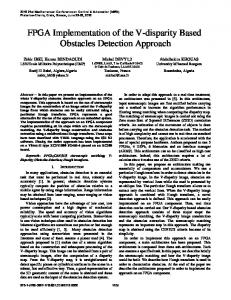
Figure 5. MAC unit. Multiplies each S coefficient by its corresponding rij value and performs a summatory among the multiplications results to obtain a unique updated rij.

Finally we need to apply once again zero flux conditions over the output of the MAC unit; it is over the evolution of rij, to model the boundary conditions of the grid boundary conditions. As with the first zero flux application we need to generate a neighbourhood of 5x5 cells. The last step is to regenerate the agent to another iteration where the diffusion takes place. The agent regeneration block simply checks the position of the current cell and in case it matches the position of the agent rij value is rewritten with its initial value, in this case the value 5, and in case it is not the agent position the rij value passes through this block and is written to r memory. This block takes 1 cycle to be performed. Now the CIR is ready to perform another iteration and so on until the total number of iterations has been reached. The initial total offset is 470 cycles. This is the number of cycles needed to full all the pipeline stages and thus to obtain the output of the first neuron of the cell grid for the first iteration. After this number of cycles a new pair of valid updated r and v values is obtained per cycle. Each iteration takes as much cycles to end as the number of neurons, in our case 3600 cycles. Besides the mentioned blocks which form the CIR neuron there is a control unit which is basically a finite state machine that controls the synchronization among the blocks, the memories, the start and end of the CIR responding to NIOS II commands and the obstacle evolution block. The NIOS II can access the memories to initialize and read them through an Altera Avalon Bus so there is also a block who acts as an arbiter over the memory data and address buses. The obstacle evolution block updates the position of the obstacle in every iteration according to a rectilinear movement (in both, x and y axis). It implements a ping-pong scheme where a couple of memories are used to store the position of the obstacle in the current iteration and the updated position for the next iteration. So while the CIR Processing block is reading from one memory the position of the obstacle in the current frame, the obstacle evolution block is updating the position for the next frame in the other memory. Once the iteration finishes, both memories swap, and so on for every iteration. In a real time implementation an MLP could be implemented to replace this block and predict complicated obstacle trajectories.

Proc. of SPIE Vol. 8068 80680J-7 Downloaded From: http://proceedings.spiedigitallibrary.org/ on 01/13/2015 Terms of Use: http://spiedl.org/terms

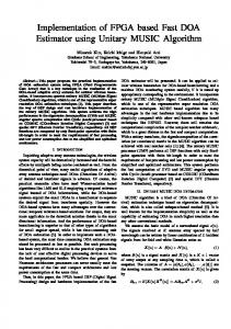
Besides the strictly implementation of the modified neuron additional tasks have to be carried out. These tasks consist on update the effective obstacles supplied to the neuron, apply Von-Neumman zero flux boundary conditions to the current cell based on the surrounding effective obstacles, create the right neighborhood for applying the mentioned zero flux and another one for the operation with the reduced version of S coefficients, apply Von-Neuman zero flux boundary conditions to the neuron outputted r variable and regenerate the agent with its initial value for the next iteration.

Figure 2. CIR block diagram.

In order to achieve an optimal CIR using this approach a small timestep must be used. The smaller the time step used the more accurate the CIR will be. Whether using small or larger timesteps, the effective obstacles will be obtained, but larger ones will affect severely the passive diffusion profile leading to poor navigation trajectories. The optimal timestep value would be 0.001 which would require a precision above 32 bits to represent the derived reduced S coefficients. In our case we have chosen a precision of 20bits which derives into a timestep of 0.1, which will be showed latter that is an acceptable value to obtain good compromise between calculation time and performance. Knowing that S coefficients have a 20bit precision, state variables r and v are signed fixed point numbers with format Q3.20, moreover memory positions storing r values expand to 28 bit words instead of 24 bit in order to store additional information of the cell like if it is a target to be reached or is a frozen cell. Once explained the modifications made to the CIR in order to be implemented on an FPGA and its overall scheme, we go on describing how one iteration is performed. There are three main steps before the incoming rij data can be computed according to dr and dv equations. The first step is updating if the cell becomes into a frozen cell or not, this is to check if the cell will be an effective obstacle by comparing rij with a value between a down and up threshold and if Oij=1. The resulting value is stored in the bit Q, which is bit 25 of r word. Down and up limits are stored in registers for quick access. Moreover the previous value of Q is added to the just calculated Q to maintain the effective obstacles frozen along the total number of iterations. This operation takes one cycle being the first stage of the neuron pipeline. The next step is to impose Von Neumann boundary conditions over the current cell, thus each cell in the obstacle boundary has the same value than that neighbour cell perpendicular to the boundary. This operation is carried out by the block zero flux. As boundary conditions are computed on the fly the block must be fed with a neighbourhood of 5x5 cells to check if the perpendicular cells are also frozen cells or toroid. This block consumes two cycles. The 5x5 neighbourhood takes as input data the serial data output from the updated frozen cells block, and with the aid of as much FIFOs as the neighbourhood order minus one, builds up a neighbourhood of 5x5 cells. Each FIFO must have at least a depth of a whole row of cells, i.e. in a grid of 60x60 it must be stored in each FIFO 60 cells. The data format 5x5 block takes care of the corners and borders, needing an initial offset of 128 cycles to output the first valid data with its neighbourhood.

Proc. of SPIE Vol. 8068 80680J-5 Downloaded From: http://proceedings.spiedigitallibrary.org/ on 01/13/2015 Terms of Use: http://spiedl.org/terms

Figure 3. From left to right blocks Q update, data format 5x5 and zero flux respectively.

Once the input data rij has been pre-processed it is ready to be fed directly to the blocks dv and dr which implements the differential equations performing its computations in parallel. vij must be delayed the right amount of cycles to arrive synchronously with its corresponding rij to dv and dr blocks.

Figure 4 shows how dv is a simple block computing the evolution of v cell state variable according to the discretized CIR equation and needs only 4 cycles to output the valid data. The dr block is responsible for the computation of the evolution of r. Inside this block it must be also evaluated the 3 degree polynomial that models a cubic non-linearity and controls the evolution of the wavefront exploring the grid. The 3 degree polynomial evaluation is solved using the Horner Algorithm, which evaluates the polynomial in 6 pipeline stages minimizing arithmetic. Uf represents the Heaviside function controlling the transition between Wave and Diffusion Regimes: when the state of the current neuron is under a threshold value, then this blocks outputs a logic ‘1’ and that neuron is subject to the active diffusion, but when is above the threshold then the blocks outputs a logic ‘0’ and the neuron state evolves according to passive diffusion.

Figure 4. From left to right blocks dv and dr respectively.

The target to be reached by the robot is represented by T which is the bit 24 of the 28 bit r word. The logic ‘and’ operation between T and r represents the reaction term, where the binary result of the operation is equal to ‘1’ if the neuron is occupied by a target and ‘0’ if not. As dr runs in parallel with dv and takes more cycles than dv to calculate its output, the control unit is responsible for controlling when to enable the writing of the updated v value to its memory and when to do the same with the updated r value. Regarding the delay dv takes 4 cycles to output first valid data while dr takes 9 cycles. The MAC unit, which is not a strictly multiply and accumulate unit, models the local coupling of the current cell with its neighbour cells. The MAC unit consumes the majority of the FPGA DSP resources invested in the design as this block performs 25 parallel multiplications and then partial sums in order to obtain a unique rij updated value. The MAC unit needs to be supplied with rij and its 25 immediate neighbours so another block to create a 7x7 neighbourhood is needed.

Proc. of SPIE Vol. 8068 80680J-6 Downloaded From: http://proceedings.spiedigitallibrary.org/ on 01/13/2015 Terms of Use: http://spiedl.org/terms

The 7x7 block is implemented in the same way as the data format 5x5 with the same kind of FIFOs but increasing its number up to 6. The data format 7x7 block and MAC unit take an offset of 191 and 6 cycles respectively to output valid data.

Figure 5. MAC unit. Multiplies each S coefficient by its corresponding rij value and performs a summatory among the multiplications results to obtain a unique updated rij.

Finally we need to apply once again zero flux conditions over the output of the MAC unit; it is over the evolution of rij, to model the boundary conditions of the grid boundary conditions. As with the first zero flux application we need to generate a neighbourhood of 5x5 cells. The last step is to regenerate the agent to another iteration where the diffusion takes place. The agent regeneration block simply checks the position of the current cell and in case it matches the position of the agent rij value is rewritten with its initial value, in this case the value 5, and in case it is not the agent position the rij value passes through this block and is written to r memory. This block takes 1 cycle to be performed. Now the CIR is ready to perform another iteration and so on until the total number of iterations has been reached. The initial total offset is 470 cycles. This is the number of cycles needed to full all the pipeline stages and thus to obtain the output of the first neuron of the cell grid for the first iteration. After this number of cycles a new pair of valid updated r and v values is obtained per cycle. Each iteration takes as much cycles to end as the number of neurons, in our case 3600 cycles. Besides the mentioned blocks which form the CIR neuron there is a control unit which is basically a finite state machine that controls the synchronization among the blocks, the memories, the start and end of the CIR responding to NIOS II commands and the obstacle evolution block. The NIOS II can access the memories to initialize and read them through an Altera Avalon Bus so there is also a block who acts as an arbiter over the memory data and address buses. The obstacle evolution block updates the position of the obstacle in every iteration according to a rectilinear movement (in both, x and y axis). It implements a ping-pong scheme where a couple of memories are used to store the position of the obstacle in the current iteration and the updated position for the next iteration. So while the CIR Processing block is reading from one memory the position of the obstacle in the current frame, the obstacle evolution block is updating the position for the next frame in the other memory. Once the iteration finishes, both memories swap, and so on for every iteration. In a real time implementation an MLP could be implemented to replace this block and predict complicated obstacle trajectories.

Proc. of SPIE Vol. 8068 80680J-7 Downloaded From: http://proceedings.spiedigitallibrary.org/ on 01/13/2015 Terms of Use: http://spiedl.org/terms

4. RESOURCES AND PROCESSING TIMES The CIR has been implemented in an Altera Stratix II EP2S60F672C3 FPGA. The blocks have been described using low level VHDL primitives with ieee.numeric_std.all library for arithmetic operations instead of ieee.std_logic_arith.all, while the place and route has been left to Altera synthesis tool Quartus II. The memories used as FIFOs involved in the creation of a 5x5 neighborhood are 64x28 bit with synchronous write and read operation. The size of the memory is determined by the number of column cells, as this memory has to store one full row, while the width of the data is determined by the width of r data plus 4 bits of additional information about the cell in that position. Four FIFOs of this kind are needed each one with a resource usage of 1792 ram bits. These memories are also used in the creation of the 7x7 neighborhood block, but in this case six FIFOs are needed. The proposed design also uses three memories to initialize and update the cell state variables, r and v, and the obstacles. State cell variables r and v memories are 28 bit and 24 bit 3600 words respectively. State r variable memory consumes 100800 ram bits while v state variable memory consumes 86400 ram bits. On the other hand obstacle memory is made up of two memories with a total 200704 ram bits consumption. The design has been synthesized and implemented using Altera Quartus II 9.1 tools. The overall system is completed with a NIOS II 32bit microcontroller targeted to control the CIR synthesized with Altera SOPC tool. A summary of the resources consumed by the whole system is depicted in Table 1.

Resources

Units

% Used

Combinational ALUTs

6,660

14

Dedicated logic registers

6,387

13

Total block memory bits

902,304

35

DSP block 9-bit elements

264

92

Total PLLs

1

17 Table 1. FPGA resources usage.

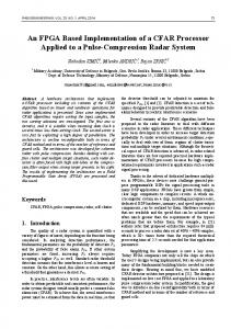
The total offset to obtain the first cell output valid data, corresponding to the cycles needed to fill all the pipeline stages and output the first iteration of the first cell data, is 470 cycles. Once this initial offset has passed, the performance of the system is to output valid data on each cycle. For valid data we mean the output of the two cell state variables and the position of the obstacle for a specific cell on a specific iteration. The CIR runs at 125 MHz and so the NIOS II microcontroller who controls it. By removing the NIOS II from the design a huge increment in the working frequency can be expected. The only way to speed up the computation is to augment the running frequency which is severing limited by the NIOS II microcontroller. A series of tests on the CIR implementation have been carried out using several obstacle schemes. The scenario resembles typical obstacles moving from one side to the other side of the arena, a robot and a target opposite to it to be reached. The objective of these tests is assessing the performance of the CIR, its right creation and if it is valid to compute the optimal trajectory to avoid the crossing obstacles.

Proc. of SPIE Vol. 8068 80680J-8 Downloaded From: http://proceedings.spiedigitallibrary.org/ on 01/13/2015 Terms of Use: http://spiedl.org/terms

Figure 6. FPGA CIR computation with a timestep of 0.1 and different obstacle scenarios.

To obtain an optimal CIR, at least 7000 iterations are needed which leads to an FPGA processing time of 0.2 seconds.

5. CONCLUSIONS A CIR implementation based on an FPGA has been proposed achieving similar results as with MATLAB model but with better performance. This architecture proposes an approach for implementing the CIR on an FPGA suitable for running a large amount of iterations with minimal delay needed to obtain a reliable Compact Internal Representation. The approach is purely sequential except in dv and dr computation which are performed in parallel. This CIR implementation is better suited for a large number of iterations and a sequential data input which the current case is. Finally it is worth to mention that it is highly encouraged to read the paper [2] to fully understand the CIR math foundation and how it is able and suitable to trace optimal trajectories for moving objects trying to avoid moving and static obstacles.

6. ACKNOWLEDGMENTS This study has been sponsored by the EU grant SPARK II (FP7-ICT-216227).

7. REFERENCES [1] Villacorta-Atienza J.A., Velarde M.G., Makarov V. “Compact internal representation of dynamic situations: Neural network implementing the causality principle”. Biol Cybem. 03, 285–297 (2010). [2] Villacorta-Atienza J.A., Salas-Paracuellos L., Alba Luis, Velarde M.G., Makarov V. “Compact Internal Representation as a Protocognitive Scheme for Robots in Dynamic Environments” Proc. SPIE (2011). [3] J.Javier Martínez-Alvarez, F.Javier Garrigós-Guerrero, F.Javier Toledo-Moreo, J.Manuel Ferrández-Vicente "High Performance Implementation of an FPGA-Based Seuqential DT-CNN". Lecture Notes in Computer Science, 2007, Volume 4528/2007, 1-9, DOI: 10.1007/978-3-540-73055-21 [4] S.Palazzo, A.Murari, G.Vagliasindi, P.Arena, D.Mazon, A. De Maack and JET EFDA contributors “Image Processing with Cellular Nonlinear Networks Implemented on Field-Programmable Gate Arrays for Real Time Applications in Nuclear Fusion” EFDA-JET-PR(10)01. [5] Zoltán Nagy, Péter Szolgay “Configurable Multi-Layer CNN-UM Emulator on FPGA” IEEE transactions 10577122 (2003).

Proc. of SPIE Vol. 8068 80680J-9 Downloaded From: http://proceedings.spiedigitallibrary.org/ on 01/13/2015 Terms of Use: http://spiedl.org/terms