Fractop: a tool for automated biological image classification David Cornforth1, Herbert Jelinek2, and Leo Peichl3 1
School of Environmental and Information Sciences Charles Sturt University, Albury, Australia Phone: +2 6051 9652 Fax: +2 6051 9897 Email:
[email protected] 2
School of Community Health Charles Sturt University, Albury, Australia Phone: +2 6051 6946 Fax: +2 6051 6772 Email:
[email protected] 3
Max-Planck-Institut für Hirnforschung Frankfurt am Main Germany Phone: +49 699 6769348 Fax: +49 699 6769206 Email:
[email protected]
Presented at the 6th Australasia-Japan Joint Workshop ANU, Canberra, Australia 30 November - 1 December 2002
ABSTRACT Biological images often contain branching structures, especially those obtained from neural tissue. Neurons are known to fall into several types, but distinguishing these types is a continuing problem. Automatic classification of neuron type relies upon suitable measurements or features. Recently fractal dimension has been suggested as a useful feature. The fractal dimension is a measure of the complexity and selfsimilarity of an image, and is becoming accepted as a feature for automated classification of images having branching structures. Fractop is a web-based program designed to assist in the analysis of such images, but is applicable to any image. Here we describe a new version of this program, which is written in Java, enabling it to be used on a variety of platforms. Fractop is able to calculate the fractal dimension of an image using five variants of the mass radius technique. We present an example showing how Fractop, in conjunction with machine learning algorithms, can be used for automated classification of rat retinal ganglion cells. Keywords and phrases: fractal dimension, branching structures, automated classification
1. INTRODUCTION Natural objects, including cells and tissues studied in pathology, have complex structural characteristics that are difficult to describe using Euclidean geometry. Biological systems experience growth that in many instances show limited self-similar properties and can be better described using fractal geometry and definable by the fractal dimension (Df). A characteristic of fractal geometry is that the length of an object depends on the resolution or the scale at which the object is measured (Mandelbrot, 1983). This dependence of the measured length on the measuring resolution is expressed as the fractal dimension of the object. The fractal dimension reflects the self-similarity or scale invariance of the object, and is given in its simplest form by
Df =
log( Ns ) log( Fm)
where Ns is the number of self similar pieces and Fm is the magnification factor. Df may be calculated in a number of ways and include the box-counting, calliper and mass-radius methods (Fernandez and Jelinek, 2001). Fractal analysis has been used in previous work to differentiate between various types of neurones in diverse species (Schierwagen, 1990; Porter and Ghosh, 1991; Jelinek and Spence, 1997; Elston and Jelinek, 2001, Jelinek and Fernandez, 2001). In this work we apply fractal analysis to the classification of rat retinal ganglion cells. These cells are particularly interesting, with cell types displaying large intra-type variation with respect to stratification level and eccentricity (Peichl, 1989). Several classification systems have been reported (see Huxlin et al., 1997; Perry, 1979, Morigiwa, Tauchi and Fukuda, 1992). Machine learning methods in conjunction with fractal analysis provide methods appropriate to the task of objectively identifying possible groupings (Jelinek and Maddalena, 1994; Karakitsos et al., 1997; Cesar and Jelinek, 2002). Automated classification is a common goal of machine learning. The object is to assign a class label to a set of observed measurements. This is achieved by determining some relationship between a set of measurements and a corresponding set of values on a nominal scale that represent the class. The relationship is obtained by applying an algorithm to a set of training samples that are 2-tuples , consisting of an input vector u and a class label z. The learned relationship can then be applied to instances of u not included in the training set, in order to discover the corresponding class label z (Dietterich and Bakiri 1995). A number of machine learning techniques including Genetic Algorithms (Holland 1992), and Neural Networks (Duda and Hart 1973) have been shown to be very effective for solving such problems. The objective of this study is to evaluate the dendritic branching patterns of rat retinal ganglion cells using several fractal dimensions, which differ in terms of their sensitivity to the global structural attributes, and classifying these with the aid of artificial learning paradigms.
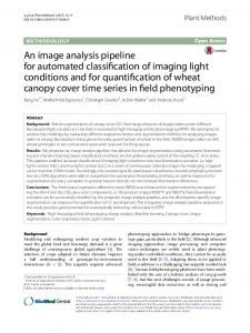
2. THE FRACTOP PROGRAM Fractop is a program written in Java, and available freely for download from the World Wide Web (http://life.csu.edu.au/~fractop). The aim of this work was to have a program with a wide accessibility in order to promote a standardisation of methods and to include a method that is sensitive to the "topological" complexity of patterns and forms. The current version of Fractop uses variations of the mass-radius method, but implementations of other methods are planned for the future. The program provides five analysis methods, which are described in more detail below. Each of the analysis methods has some common image pre-processing code that produces an array of the “on” pixels within the image. The common code calculates the centre of mass of the image and the radius of gyration about that centre. This is multiplied by a factor between zero and one, and within this smaller radius, a number of centres are chosen. The factor determines how widely spaced the centres are. In Fig. 1 the smaller radius is shown by a solid line and the centres are indicated by concentric circles. This leads to a varying number of image points being used as centres depending on the covering factor of the image. The radius of gyration or a fraction thereof may lead to centres being closer together but the main purpose is to restrict the analysis to the central regions of the image where scale-invariance is more likely to be present (in the case of neurons) (Caserta and Eldred, 1995). The methods fall into two main areas: the cumulative mass method and the cumulative intersection method. The first of these methods counts the cumulative number of pixels Mc in the image occurring at each radius r from some centre point:
Df =
log( M c ) log(r )
The second method counts the cumulative number of intersections Ic between image line segments and circles of increasing radii r:
Df =
log( I c ) log(r )
2.1 Mass-radius analysis The mass-radius method is the simplest algorithm to implement, and follows the method of Caserta and Eldred (1995). The fractal dimension is defined by the relationship between the area of the image found within a certain radius covering the image. The area M increases with the increase in the radius r according to
M = µr d For strictly self-similar mathematical fractals the mass dimension is the same as the Hausdorff dimension (Schroeder, 1991). Circles are placed at randomly generated centres within a fraction of radius of gyration, and the radius of each circle is incremented by one pixel at each step. This produces a series of expanding concentric circles, as shown in Fig. 1. The number of pixels contained in each circle is counted at each step. The analysis ceases when the edge of the image is reached and no pixels of the image are encountered. The cumulative sum of pixels is calculated for each radius. The slope of the log-log relationship between cumulative mass and radius is calculated by linear regression, and the gradient gives the fractal dimension
Fig. 1. The arrangement of centres used in the calculation of fractal dimension using the mass radius method.
2.2 Cumulative Intersection Analysis This method, like the mass-radius method, uses the circles randomly generated within the fraction of the radius of gyration. The cumulative intersection method was developed by Schierwagen (1990), based on the method described by Sholl (1953). For each centre, the radius of the circle is increased by one pixel at each step. The number of separate branches is counted for each radius. This is done as follows. The points are sorted by radius and by angle for points of equal radii. The sorted array is then traversed in order and if two consecutive points of the same radius are not adjacent, the intersection count for that radius is incremented (see Fig. 2). Adjacent points, including points on the diagonal, are those points touching each other. Computationally, adjacency holds when the sum of the absolute differences of the x and y coordinates respectively is less than or equal to 2. Note, that adjacent points will be part of the same branch and hence, an intersection should not be counted.
Fig. 2. A small section of an image is shown, with a single circle corresponding to the radius selected at some point during analysis. Consecutive points that are also adjacent are indicated by A, while consecutive points that are not adjacent are indicated by B.
The analysis ceases when the edge of the image is reached and no branches are found. The cumulative number of branches is calculated. The slope of the log-log relationship between cumulative number of intersections and radius is calculated by linear regression, and the fractal dimension obtained as previously described.
2.3 Convex hull mass radius analysis The convex hull method (Sedgewick 1992) uses a convex hull instead of a set of circles. This involves initial computation of a convex hull bounding the extremities of the cell image (Fig. 3). The hull is then scaled, so that at each step, the size of the hull is increased by one pixel, and the number of pixels incident with this hull are counted. The convex hull method is an attempt to handle self-affine fractals in a more appropriate manner.
Fig. 3. Showing a convex hull (dotted line) of the image.
2.4 Convex hull intersection analysis 3. This method uses the same convex hull (Fig. 3), but counts intersections in a manner similar to the other intersection methods described above.
2.5 Vectorised Intersections The vectorised intersection method is an adaptation of the cumulative intersection method to vector images. The input raster image is first vectorised producing a thinned image, and a series of nodes where component lines meet. From these nodes, line segments are extracted and removed recursively starting at terminal nodes. Terminal nodes have only one line branching from them. This process is repeated until no nodes, and hence lines, remain. Analysis is then performed on a line-by-line basis, with each line segment falling into one of two analysis categories with respect to the centre point. The first category applies to lines whose end-points subtend an angle of less than 90 degrees to the centre point (Fig. 4a). In this case, there exists only one point of intersection between the line and any circle with a radius between the radii of the two end points. The second category applies to lines whose endpoints subtend an angle of greater than 90 degrees to the centre point (Fig. 4b). The radii of the two end points are calculated, as well as the perpendicular distance of the centre point from the line. This distance will correspond to the circle of minimum radius that intersects the line. Between this minimum radius and the smaller of the two end point radii, we count two intersections. For radii between the two end point radii, we count only one intersection. The number of intersections is acquired in a similar way to the cumulative intersections method, and the stopping criteria are the same.
a)
b)
Fig. 4. a) Line segments whose end-points subtend an angle of less than 90 degrees count as one intersection. b) Line segments whose end-points subtend an angle of greater than 90 degrees count as two intersections.
3. METHODS Images were obtained from 85 rat retinal ganglion cells using histological techniques as described in Peichl (1989). The resulting images were classified by inspection, and divided into groups based on stratification (inner (i) or outer (a) part of the inner plexiform layer of the retina) and type (α or δ) as summarised in Table 1. type strat Total a 27 10 37 i 44 4 48 Total 71 14 85 Table 1. A summary of the 85 cells used in the experiments. δ
α
From these images we calculated lacunarity and 4 additional metric variables: • • • •
The surface area of cell in microns The eccentricity, or distance of the cell from the place of highest cell density in retina, measured in mm. The dendritic area measured in mm The maximum dendritic diameter in microns
The Fractop program was used to calculate fractal dimension using the five different methods described above, providing a total of 11 features. The parameters used in Fractop were radius factor = 0.33 and number of centres = 20. We used the features as the basis for automated classification procedures to identify differences between stratification and type. A number of automated classifier algorithms are available using the excellent Weka toolbox (Witten, and Frank, 1999). These are briefly discussed below and include Nearest Neighbours (IB1 and Ibk), Naïve Bayes, Decision Tree Induction and Decision Table. The nearest neighbour algorithm (Fisher, 1936) simply stores samples. When an example is presented to the classifier, it looks for the nearest match from the examples in the training set, and labels the unknown example with the same class. An extension is to look at the nearest k neighbours. We have used this algorithm with k=1 and k=3. The naïve Bayes algorithm (Bayes, 1763) assumes that attributes are independent. From the correlation analysis above, we know this is untrue, but the algorithm performs surprisingly well. It estimates prior probabilities by calculating simple frequencies of the occurrence of each attribute value given each class, then returns a probability of each class, given an unclassified set of attributes. The decision tree induction algorithm (Quinlan, 1986) uses the C4.5 algorithm to form a tree by splitting each variable and measuring the information gain provided. The split with the most information gain is chosen as the first split, then the process is repeated until the information gain provided is below a threshold.
We also used an implementation of the Cerebellar Model Articulation Controller (CMAC) (Albus, 1975) with the kernel addition training algorithm (Cornforth and Newth, 2001). This algorithm divides the input space using multiple overlapping grids and builds a probability density function for each class. An unknown input can then be associated with an appropriate probability value for each class. The input is assigned to the class having the largest probability. These algorithms were given three classification tasks. In the first, data were divided into four groups based on stratification and type. In the second task, data were divided into the groups of based on stratification alone. In the third task, data were divided into groups based on type alone. The performance of the algorithms was tested using ten-fold cross validation in order to avoid over fitting of the model (Weiss and Kulikowski 1991). The data sets used were each divided into ten parts at random. Training was performed using nine parts of the data, and the trained model was tested on the remaining one part. This was done ten times using a different part for testing. In this manner, each model was tested on all data, and reported a number of correctly classified records. The results are compared to a default classifier, where the class most frequent in the data is chosen.
4. RESULTS Fractop was able to produce measures of fractal dimension, obtained by five different methods, for each of the 85 cells, in less than an hour. A summary of these values is given in Table 2. The values obtained showed some differences between the different types and stratifications of cells, but the largest differences were found between values obtained using the mass-radius and intersection methods. strat / type Total strat / type Total a 1.513 1.525 1.516 a 1.675 1.681 1.677 i 1.526 1.537 1.527 i 1.680 1.691 1.681 Total 1.521 1.528 1.522 Total 1.678 1.684 1.679 (a) (b) Table 2. Average values of Fractal Dimension obtained from Fractop using (a) Mass Radius methods and (b) intersection methods. δ
α
δ
α
The results of the machine learning are shown in table 3. For the first classification task, the 4-class problem, the lowest rate was 52% for the nearest neighbours method, which is no better than the default classifier. The best performance was 66%, achieved by the Naïve Bayes and CMAC methods. For the second task, classifying type proved an easy task for the default classifier, as there were 71 cells of type α, compared to only 14 of type δ. The machine learning algorithms managed 88% correct. For the third task, the machine learning techniques did extremely well, lifting the correct classified rate from 56% for the default classifier to 92% using the Naïve Bayes classifier. As can be seen, the stratification is easy to classifier while the type is less so. type and strat type strat 52% 84% 56% Default 66% 74% 92% NaiveBayes 52% 88% 55% IB1 55% 88% 67% IBk-3 60% 85% 81% j48.J48 59% 87% 73% Dec.Table 66% 88% 72% CmacKata Table 3. Results from the automated classification tests using the machine learning methods indicated, and described in the text.
5. DISCUSSION These results demonstrate the usefulness of Fractop as a means of calculating fractal dimension for a variety of medical images. However, Fractop can be applied to images in many other areas. Since this program is freely downloadable from the Internet, it is of benefit to researchers all over the world. These preliminary results from the machine learning methods suggest that one method is not sufficient to guarantee a clear distinction between different types and stratifications of rat retinal ganglion cells. Previous
work has suggested that machine learning algorithms are superior to linear and quadratic discriminant functions or logistic regression analysis (Einstein et al., 1998) and several of these algorithms were applied in our study. Cells in different stratification levels could be distinguished using these machine-learning methods, when fractal dimension was combined with other standard measures. Distinguishing the type was also possible, but was obscured by the imbalance in the numbers of samples from each class. Our results suggested that a combination of techniques would be preferable, and that further work is required in the choice of features to be used. The differences observed between the Dfs obtained using the cumulative intersection method compared to the mass-radius method agreed with the results reported by Chialvo et al. (1991) for thalamic neurons. These authors compared the cumulative intersection method to the box-counting method. In both studies, the cumulative intersection method gave higher Dfs but differentiated between neuron types. This suggested that the various fractal analysis methods are sensitive to different morphological features of an image and cannot be directly compared to each other. Rather, they are separate measures, which in combination define an image. Fractop is a new method for obtaining fractal dimension of images. The benefits are that it is downloadable anywhere, and multi-platform friendly.
ACKNOWLEDGEMENTS We wish to acknowledge the work of Tony Steinke and Peter Bowdren, who worked on the first version of Fractop, and Cherryl Kolbe and Bev De Jong for technical assistance with preparing the images of the cells.
REFERENCES Albus, J. S. (1975). A New Approach to Manipulator Control: the Cerebellar Model Articulation Controller (CMAC). Trans. ASME, Series G. Journal of Dynamic Systems, Measurement and Control. 97, 220-233. Bayes. T., 1763, An essay towards solving a problem in the doctrine of chances. Philosophical Transactions of the Royal Society of London 53:370-418. Caserta, F. and Eldred, D. (1995). “Determination of fractal dimension of physiologically characterized neurons in two and three dimensions.” Journal of Neuroscience Methods 56: 133-144. Cesar, R.M., Jr. and Jelinek, H.F. (2002) Segmentation of retinal fundus vasculature in non-mydriatic camera images using wavelets. In: Angiography Imaging: State-of-the-Art Acquisition, Image Processing and Applications Using Magnetic Resonance, Computer Tomography, Ultrasound and X-rays. Eds. Suri, J. and Laxminarayan. T., Chapter 9. Academic Press, N.Y. (in print) D. Chialvo, C. Vahle-Hinz, K.D. Kniffki and A.V. Apkarian. (1991) Fractal dimension of neurons located in the cat's thalamic ventrobasal complex (vb) and its ventral periphery (vbvp)". Neuroscience Society, 17(1): 622. Cornforth, D. and Newth, D. (2001). The Kernel Addition Training Algorithm: Faster Training for CMAC Based Neural Networks. Proc. Conf. Artificial Neural Networks and Expert Systems, Otago. Dietterich, T.G. and Bakiri, G. (1995). Solving Multiclass Learning Problems Via Error-Correcting Output Codes. Journal of Artificial Intelligence Research, 2: 263-286. Duda, R.O and Hart, P.E. (1973). Pattern Classification and Scene Analysis. New York: John Wiley and sons. Einstein AJ. Wu HS. Sanchez M. and Gil J. (1998) Fractal characterisation of chromatin appearance for diagnosis in breast cytology. Journal of Pathology. 185(4):366-381. Elston, G.N. and Jelinek, H.F. (2001) Pyramidal neurons in the visual cortex of the New World marmorset monkey (Callithrix jacchus). A study of dendritc branching patterns with comparative notes on the Old Word macaque monkey (Macaca Fasicularis). Fractals, 9(3):297-304. Fernandez, E. and Jelinek, H.F. (2001) Use of fractal theory in neuroscience: methods, advantages and potential problems. Methods, 24(4):309-321. Fisher, R.A., (1936). The use of multiple measurements in taxonomic problems. Annual Eugenics 7 (part II):179188. Reprinted in Contributions to Mathematical statistics, 1950, Wiley.
Holland, J. (1992). Adaptation in Natural and Artificial Systems: An Introductory Analysis with Applications to Biology, Control, and Artificial Intelligence. MIT Press, second edition. Huxlin, K. R. and A. K. Goodchild (1997). “Retinal ganglion cells in the albino rat: revised morphological classification.” The Journal of Comparative Neurology 385: 309-323. Jelinek, H.F. and Fernandez, E. (2001) Use of fractal theory in neuroscience: methods, advantages and potential problems. Methods, 24(4):309-321. Jelinek, H.F. & Maddalena, D.J. (1994). Application of artificial neural networks to cat retinal ganglion cell categorization. In: Tsoi, A.C. & Downs, T. (Eds.). Proceedings of the fifth Australian conference on neural networks: University of Queensland, Brisbane. Jelinek, H.F. and Spence, I. (1997) Categorisation of physiologically and morphologically characterised nonalpha / non-beta cat retinal ganglion cells using fractal geometry. Fractals, 5(4):673-684. Karakitsos, P., Stergiou, E.B., Pouliakis, A., Tzivras, M., Archimandritis, A., Liossi, A. and Kyrkou, K. (1997) Comparative study of artificial neural networks in the discrimination between benign from malignant gastric cells. Analytical & Quantitative Cytology & Histology. 19(2) 145-152. Mandelbrot, (1983) The Fractal Geometry of Nature. W.H. Freeman and Co., New York. Morigiwa, K., M. Tauchi and Y Fukuda. (1992) Morphological comparisons between outer and inner ramifying alpha cells of the albino rat retina. Experimental Brain Research, 88: 67-77. Peichl, L. (1989). “Alpha and delta ganglion cells in the rat retina.” The Journal of Comparative Neurology 286: 120-139. Perry, V. H. (1979). “The ganglion cell layer of the retina of the rat: a Golgi study.” Proc. R. Soc. London B 204: 363-375. Porter, R., S. Ghosh, et al. (1991). “A fractal analysis of pyramidal neurons in mammalian motor cortex.” Neurosscience Letters 130: 112-116. Quinlan, J.R., 1986, Induction of Decision Trees. Machine Learning, 1(1):81-106. Schierwagen, A. (1990). "Scale-invariant diffusive growth: a dissipative principle relating neuronal form to function". In J. Maynard-Smith and G. Vida, editors, Organisational constraints on the dynamics of evolution, pp. 167-189, Manchester University Press. Schroeder, M. (1991). Fractals, Chaos, Power Laws: Minutes from an Infinite Paradise. W H Freeman & Co. Sedgewick, R (1992). Algorithms in C++. Addison-Wesley, USA. D.A. Sholl (1953). Dendritic organization in the neurons of the visual cortices of the cat. Journal of Anatomy, 87:387-406, 1953. Weiss and Kulikowski, (1991) Computer Systems That Learn. Morgan Kaufmann. Witten, I.H. and Frank, E.: (1999). Data Mining: Practical Machine Learning Tools and Techniques with Java Implementations. Morgan Kaufmann