p and d represent the 2D locations of pixels and disparity, and I is a vector with RGB color. We compute the per-pixel cost e(p, d) with the el, et. When computing ...
Freeview rendering with trinocular camera Dongbo Min, Donghyun Kim
SangUn Yun
Kwanghoon Sohn
Dept. of Electrical and Electronic Engineering, Yonsei University, Seoul, Korea
Samsung Electronics, Suwon, Korea
Dept. of Electrical and Electronic Engineering, Yonsei University, Seoul, Korea
y
Abstract— The paper presents a method for synthesizing novel view from the virtual camera with trinocular camera configuration. We propose a cost aggregation method with weighted least square for stereo matching, and address the occlusion problem by using cost functions computed with multiview images. We avoid the redundancy of estimating disparity maps for all the images by using simple geometry transfer method. The novel view is synthesized by view-dependent geometries on the 3D translation of virtual camera. Experimental results show that the proposed method yields the accurate disparity maps and the synthesized novel view is satisfactory enough to provide a viewer freeview videos.
Top view
Left view
x
978-1-4244-1684-4/08/$25.00 ©2008 IEEE
Center view
( B,0,0)
: Movement volume of virtual camera
I. I NTRODUCTION For decades, the problem of synthesizing the novel views with a limited number of the cameras has been an important issue in the field of computer vision, and many methods have been proposed to solve this problem in the area of image-based rendering (IBR). Novel view rendering is one of the most important techniques in the free viewpoint television (FTV), which provides the reality and interactivity by enabling a viewer to select the viewpoint. Imagebased rendering can be classified into three categories according to the estimation of geometry information: rendering without geometry, rendering explicit geometry, and rendering with implicit geometry. Light field and lumigraph approaches use the rendering without geometry which performs the photorealistic rendering with just a simple planar geometry representation [1][2]. However, a significant number of 2D images should be used to reconstruct a function that defines the flow of light through the 3D space. A second group of researches reconstruct the complete 3D model from the 2D images and render the model from the desired viewpoint. The difficulties of generating the complete 3D model cause these approaches to be applied in the limited applications only [3]. The rendering with implicit geometry synthesizes the novel views from the virtual camera which is located between the captured views by using a small number of cameras. The reference images are warped by the geometry information, and the novel view are compute by the weightedinterpolation. A number of view interpolation approaches have been proposed to improve the performance [4][5][6]. In this paper, we propose a new method of synthesizing novel views from the virtual camera based on sparsely sampled reference images. In order to extend a dimension of the viewpoint where virtual view is synthesized, we use a trinocular camera configuration which consists of the center, left and top cameras, as shown in Fig. 1. While camera movement in the conventional method is usually limited to x-axis, the proposed method can synthesize the novel view in 3D volume, that is, in the x, y, and z axes. The N -view & 1-depth framework is used to reduce the redundancy on the disparity estimation. In this framework, we can estimate the accurate disparity map on the center image with multiview images to address the occlusion problem, which has the significant effects for novel view rendering. Then, the disparity maps on the left and top images are computed by transferring the geometry information on the center image, so that we can perform the novel view rendering efficiently and correctly.
z
(0, B,0)
Fig. 1.
Trinocular camera configuration.
II. T RINOCULAR S TEREO MATCHING We use the trinocular camera configuration for estimating the disparity and rendering virtual view, as shown in Fig. 1. We assume that the baseline distances from the center image are B. The novel view from the virtual camera can be synthesized in the volume which is encircled by the dotted lines. A. Per-pixel cost computation When estimating the disparity field, two or more images are used. The difference image is computed for center view. Since the multiple images are rectified into horizontal (or vertical) direction, we obtain the difference image by shifting the left (or top) image to the right (or lower) direction, and the subtracting the center and shifted left (or top) images. el (p, d) = |Ic (x, y) − Il (x + d, y)| (1) et (p, d) = |Ic (x, y) − It (x, y + d)| p and d represent the 2D locations of pixels and disparity, and I is a vector with RGB color. We compute the per-pixel cost e(p, d) with the el , et . When computing the per-pixel cost, we should consider whether corresponding pixels in the reference images is visible or occluded. We assume that there exists at least one visible point for all the pixels in the center view. For left (or top) image, the occluded pixels usually exist in the right (or lower) part of an object in the center image. The assumption is useful for handling occlusion, although it is invalid in a few pixels, especially, in the lower right parts of the center image. Based on the principle which the matching cost of visible pixel is generally smaller than that of occluded pixel, we compute the final cost function on the center image as follows: e(p, d) = min(el (p, d), et (p, d))
(2)
While most approaches detect the occlusion regions by using uniqueness constraint and assign pre-defined values to the occluded pixels, we address the occlusion problem with multiview images in the process of computing cost function. B. Proposed cost aggregation In order to estimate the optimal cost E(p, d), we use a prior knowledge that costs should vary smoothly, except at object boundaries.
3446
Stereo image pairs
From this observation, we are able to estimate the cost function by minimizing the following energy model with weighted least square: ε(E) =
Per-pixel cost Computation
2
(E(p) − e(p)) dp wp,p+n (E(p) − E(p + n))2 +λ Ω +wp,p+n⊥ (E(p) − E(p + n⊥ ))2 n∈N1 N1 = {(xn , yn )|0 < xn ≤ M, 0 ≤ yn ≤ M } Ω
dp
(3)
e0 (d )
2
, where w represents the weighting function between corresponding neighbor pixels. We simplify E(p, d) to E(p), since the same process is performed for each disparity. n and n⊥ represent the 2D vectors, which are perpendicular to each other. M represents the size of a set of neighbor pixels. Taking the first derivative of Eq. (3) with respect to E, we obtain the following equation: E(p) − e(p) +λ n∈N1
wp,p+n (E(p) − E(p + n)) −wp−n,p (E(p − n) − E(p)) +wp,p+n⊥ (E(p) − E(p + n⊥ )) −wp−n⊥ ,p (E(p − n⊥ ) − E(p))
=0
(4)
To simplify the above equation, we redefine the set of neighbor pixels. When p is (x, y), the set can be expressed as: N (p) = {p + pn | − M ≤ xn , yn ≤ M, xn + yn �= 0} By using the above notation, Eq. (4) is expressed as: wp,m (E(p) − E(m)) = 0
E(p) − e(p) + λ
(5)
m∈N(p)
The solution of the (k + 1)th iteration is obtained by the following equation: ¯ k (p) E k+1 (p) = e¯(p) + E e(p) + λ
wp,m E k (m) m∈N(p)
=
1+λ
(6)
wp,m m∈N(p)
Eq. (6) consists of two parts: normalized per-pixel matching cost and weighted neighboring pixel cost. By running the iteration scheme, the cost function E is regularized with the weighted neighboring pixel cost. In the proposed method, we use the Gaussian weighting function with the CIE-Lab color space in Eq. (7). rc and rs are weighting constants for the color and geometric distances, respectively. It is necessary to use the term for geometric distance in the weighting function, since the smoothness constraints with more neighborhoods are considered. c Cp,m Sp,m wp,m = exp − 2r 2 + 2r 2 c s c (7) Cp,m = (Lcp − Lcm )2 + (acp − acm )2 + (bcp − bcm )2 Sp,m = (p − m)2
e1 (d )
e2 (d )
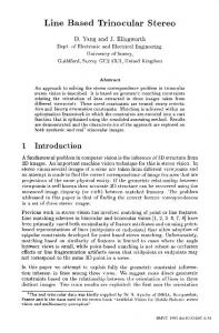
Fig. 2.
Cost aggregation
m∈Nc (p)
1+λ
m∈Nn (p)
wp,m m∈N(p)
wp,m E k (m) (8)
E1 (d ) Adaptive Interpolation
E2 ( d )
Overall framework of the proposed cost aggregation.
2) Multiscale Approach: As previously mentioned, it is necessary to gather pixel information at a large distance to ensure reliable matching. This implies that a number of iterations are required to estimate the correct cost function. We use a multiscale approach to solve this problem. Our method is different from the conventional approaches in the sense that it is applied in the cost domain. In Eq. (8), the cost function E(p) can generally be initialized to e(p). We can initialize the value close to the optimal cost in each level by using the final value in the coarser level. Using Eq. (8), the proposed method performs cost aggregation independently in each section with the same disparity of the 3D cost volume. Conventional multiscale approaches reduce image resolution at first, and then the estimation process continues. The reduction of the resolution also reduces the search range of the disparity. For instance, if we use the multiscale approach over three levels, the search range will have been reduced to a quarter of the original search range on the coarsest level. Thus, two cost functions in the finer level Ef (p, 2d) and Ef (p, 2d+1) are initialized by using the cost function in the coarser level Ec (p, d). To avoid this problem, we use an alternative multiscale scheme for cost aggregation. We first compute the 3D cost volume and then perform the proposed multiscale scheme in each 2D cost function. The proposed multiscale method runs the iterative scheme at the coarsest level by initializing the cost function to e(p, d). After K iterations, the resulting cost function is used to initialize the cost function in the finer level, and this process is repeated until the finest level is reached. The proposed multiscale scheme is shown in Fig. 2, which includes adaptive interpolation. When the cost function on the (l+1)th level is defined as El+1 (p), we can refine the resolution of the cost function El (p) on the finer level by using bilinear interpolation. However, if bilinear interpolation is used, the error can be propagated into the neighborhood regions, especially on the boundary region. To avoid this problem, we propose an adaptive interpolation method based on the weighted least square: el (p) + λa
1) Gauss-Seidel Acceleration: One reason for slowing down the convergence in Eq. (6) is that the updated components in each pixel are used only after one iteration is complete. We compensate for this problem by using the updated components in each pixel intermediately. We divide a set of neighbor pixels N (p) into two parts: the causal part Nc (p) and the non-causal part Nn (p). Eq. (6) is expressed as follows, based on this relationship:
=
Cost aggregation
2
C. Acceleration Scheme
¯ k (p) E k+1 (p) = e¯(p) + E wp,m E k+1 (m) + λ e(p) + λ
Adaptive Interpolation
E0 (d )
El (p) =
pm ∈N(pi )
1 + λa
wp,pm El+1 (pm )
pm ∈N(pi )
wp,pm
(9)
, where pi = (xi , yi ) represents a pixel on the coarser level, and N (pi ) on the (l + 1)th level is a set of 4-neighboring pixels. In Eq. (9), w represents the weighting function, equivalent to that in Eq. (6). We set the weighting factor to λa = 15. Another advantage of adaptive interpolation is to increase the resolution of the cost function so that no blocking artifact exists. The adaptive interpolation by the intensity values on two successive levels leads to the up-sampling scheme, which preserves the discontinuities on the boundary region. Thus, it is not necessary to perform the cost aggregation scheme on the finest level, and this makes the proposed method faster.
3447
III. V IRTUAL VIEW RENDERING A. N-view & 1-depth framework We estimate the disparity map on the center image by using the proposed cost aggregation method, and handle the occlusion problem based on the computation of the cost function with multiview images. It is necessary to acquire N depth maps (in this paper, N is 3) for rendering the novel view in the trinocular camera configuration. Since all the images are rectified, the disparity maps in the left and top image are equivalent to that of the center image, except some regions such as occluded region in two images. Instead of estimating the disparity maps on the left and top images with the proposed cost aggregation method, we propose the approach of computing them by transferring the disparity map on the center image. Then, the extrapolation method is used to fill the disparity on the occluded region in the left and top images. Since the occluded pixels are usually included in the background, we assign reasonable disparity value to the occluded pixels with the background disparity. In other words, the extrapolation is done from the left to the right parts in the left image, and from the upper to the lower part in the top image. Therefore, it is possible to acquire the disparity maps for all the images asymmetrically only with trivial additional computational loads. B. Novel view generation 1) Projection of reference images: The virtual view can be synthesized by warping each image with its disparity map. All the images are warped and the novel view is synthesized by performing the weighted-interpolation. The way of synthesizing novel views from virtual camera is as follows: 1. Perform back-projection for all the pixels in the reference image into 3D space by using the disparity map. 2. Transform the coordinate of the reference camera into the coordinate of the virtual camera. 3. Perform the projection of 3D points into image plane of the virtual image. Using the above process, the texture in reference image is mapped into novel view from virtual camera. The process is done for all the reference images. Since all the images are rectified, the viewing directions are same, in other words, there exists only translation between cameras. The rotation of the virtual camera is not considered in the novel view rendering, since the rotation of the virtual camera causes a number of holes in the novel view and it is not appropriate in video-conferencing or 3DTV. A point mc (xc , yc ) with disparity dc on the center image is converted into 3D point Mc as follows: (xc − x0 )B (yc − y0 )B f B , , (10) dc dc dc , where (x0 , y0 ) is the center of the image plane. When the virtual camera has the translation (Tx , Ty , Tz ), we can compute the 3D point Mv in the virtual camera coordinate: (yc − y0 )B fB (xc − x0 )B + Tx , + Ty , + Tz dc dc dc
(11)
By projecting the 3D point Mv into image plane of the virtual camera, we can acquire the relation between the corresponding pixels in the reference and virtual images. A point in the novel view mn (xn , yn ) can be computed as follows: 0 )B/dc +Tx xn − x0 = f (xc −x = f B/dc +Tz
yn − y0 = f
(yc −y0 )B/dc +Ty f B/dc +Tz
=
xc −x0 +dc αx 1+dc αz /f yc −y0 +dc αy 1+dc αz /f
(12)
To simplify the notation, we use a normalized coordinate (αx , αy , αz ) = (Tx , Ty , Tz )/B, and set the baseline distance to 1. By using the similar process, we can also induce the relations in the left and top views. xn − x0 = yn − y0 =
xl −x0 −dl (1−αx ) 1+dl αz /f yl −y0 +dl αy 1+dl αz /f
xn − x0 = yn − y0 =
xt −x0 +dt αx 1+dt αz /f yt −y0 −dt (1−αy ) 1+dt αz /f
(13)
Let Ii and Ini the reference and projected images, respectively, then Ini (xn , yn ) = I i (xi , yi ), i = c, l, t. When the novel view with forward warping is synthesized, there may be some problems. Since the relation in Eq. (12) and (13) is not one-to-one mapping, multiple projections and holes in the novel view usually exist. The multiple projections into the novel view can be caused by two reasons: depth discontinuity and image resampling. The pixels on the depth discontinuities are projected into the same point in the novel view, although they have different disparities (depths). In this case, the pixel that has the largest value of disparity among the projected pixels should be retained since the pixel should cover the remaining pixels of objects which are farther from the camera. Another problem is due to image resampling. When the objects zoom out (or in) in the novel view rendering, there may be the multiple projections (or holes), although they are equal disparity values. Moreover, the point (xn , yn ) in the novel view may not be integer form. In order to solve these problems, we adopt the backward warping and bilinear interpolation in the novel view rendering. Given the novel viewpoint, we perform the geometry resampling in the novel view, by transferring the depth and occlusion information to the novel view for each reference image. Simple median filtering is performed in the depth and occlusion map to eliminate small holes. The backward warping prevents the quality of the novel view from being degenerated by the image resampling. Since it is known that disparity varies smoothly, geometry resampling does not affect the quality of novel view rendering, different from image resampling. 2) Error-compensated view interpolation: The final reconstructed novel view is computed by an adaptive interpolation with the projected images. The quality of the projected images is usually different from one another, since the quality depends on the disparity maps of the reference images. To compensate the error which can be generated for disparity estimation and geometry resampling, we propose the adaptive view interpolation considering the compensation error. The adaptive interpolation is a weighted-average as follows: In (p) =
wl (p, α)Inl (p) + wc (p, α)Inc (p) + wt (p, α)Int (p) wl (p, α) + wc (p, α) + wt (p, α)
(14)
, where α(αx , αy , αz ) is 3D locations of virtual camera, and wi (p, α) is a weighting factor which is related to the quality of the projected image, the visibility of a pixel and the location of virtual camera. The quality of the projected image is measured by using relative rate of compensation errors Ccl , Cct , and Clt . Ccl = |Inc − Inl |, Inc ,
Inh ,
Inv
Cct = |Inc − Int |,
Clt = |Inl − Int |
are the corresponding points of three reference images, respectively. The weight for the projected image should be high, when its disparity compensation errors are small. Based on the above discussion, a weighting factor that is related to the quality of the projected image Qc (p) is defined as follows: Ccl + Cct Clt = (15) Qc (p) = 1 − Ccl + Cct + Clt Ccl + Cct + Clt Qc represents a quality-weighting factor for the center image, and the weighting factors for left and top images are also defined in the similar process. The final weighting factors are defined as follows:
3448
Fig. 4. Results for (from left to right) left, center, and top images of a set of ‘Mans’ images.
Fig. 3. Results for (from top to bottom) ‘Tsukuba’, ‘Venus’, ‘Teddy’ and ‘Cone’ image pairs: (from left to right) original images, ground truth maps, our results, error maps.
wl (p, α) = Vl (p) · (Ql (p) + K) · αx wc (p, α) = Vc (p) · (Qc (p) + K) · (1 − αx − αy ) wt (p, α) = Vt (p) · (Qt (p) + K) · αy
Fig. 5.
(16)
V (p) is a visibility function whether a pixel in the novel view is visible in the reference views, and 1 (or 0) when visible (or not). K is a offset parameter, and set to 0.2. IV. E XPERIMENTAL RESULTS To validate the performance of the proposed stereo matching, we performed the experiments with the Middlebury test bed [7]. We use the following test data sets: ‘Tsukuba’, ‘Venus’, ‘Teddy’, and ‘Cone’. Since the test data sets are provided for two-view stereo algorithm, we performed the stereo matching with left and right images, instead of the trinocular stereo images. The proposed method is tested using the same parameters for all the test images. The two parameters in the weighting function are rc = 8.0, rs = 8.0, and the weighting factor is λ = 1.0. We use the multiscale approach at four levels, and the number of iterations is (3, 2, 2, ×), on a coarse to fine scale. The iteration number of the finest level is not defined since we use the adaptive interpolation technique in the upsampling step, as mentioned in section II. The sizes of the sets of neighbor pixels are 5 × 5, 7 × 7, 9 × 9, and 9 × 9. Fig. 3 shows the results of the proposed method for the test bed images. The proposed method yielded accurate results for the discontinuity, occluded, and textureless regions. Since only two images are used in stereo matching, we cannot address the occlusion problem, so that the occlusion handling approach proposed in [8] was applied to acquire the final disparity map. Since we used the trinocular stereo images for novel view rendering, the occlusion handling approach proposed in [8] was not used in other test images. Fig. 4 shows the results of the trinocular stereo images ‘Mans’ used in the experiments. The ‘Mans’ image, as captured by the Digiclops camera of Point Grey Research Inc., has very complex geometry and large occluded region. The test image has the size of 640 × 480, and the search range is 35. We could find that the disparity maps on the left and top images were accurate and had good localization on the object boundary, although these were computed by simple transfer and extrapolation techniques. Fig. 5 shows the synthesized novel images from the virtual camera. We could find that the natural
Synthesized novel views.
images were synthesized in the object boundary and occluded region. The quality of the synthesized images were satisfactory enough to provide a user the seamless videos for FTV. We can also provide the stereoscopic images, which consists of the left and right synthesized views. The synthesized videos are available at [9], which are 2D and 3D stereoscopic videos. V. C ONCLUSION In this paper, we have presented the new approaches of synthesizing the novel view from the virtual camera. The disparity map which was estimated by the proposed method was accurate and robust to occlusion problem. We could synthesize the novel view seamlessly on the 3D translation of virtual camera. In further work, we will develop the general novel view rendering system by using the proposed system as the basic unit in the multiview camera configuration, and investigate the backward warping method which is more robust to error of disparity map. ACKNOWLEDGMENT This research was partially supported by the MIC, Korea, under the ITRC support program supervised by the IITA, and was partially supported by the IT R&D program of MIC/IITA. R EFERENCES [1] M. Levoy and P. Hanrahan, “Light field rendering,” SIGGRAPH, pp. 3142, 1996. [2] S.J. Gortler, R. Grzeszczuk, R. Szeliski and M.F. Cohen, “The lumigraph,” SIGGRAPH, pp. 43-54, 1996. [3] Paul E. Debevec, Camillo J. Taylor, and Jitendra Malik, “Modeling and rendering architecture from photographs: a hybrid geometry- and imagebased approach,” SIGGRAPH, pp. 11-20, 1996. [4] Chen, E. and Williams, L., “View interpolation for image synthesis,” SIGGRAPH, pp. 279-288, 1993. [5] L. Zhang, D. Wang, and A. Vincent, “Adaptive Reconstruction of Intermediate Views From Stereoscopic Images,” IEEE Trans. CSVT, vol. 16, no. 1, pp. 102-113, Jan. 2006. [6] L. Zitnick and S. Kang, “Stereo for Image-Based Rendering using Image Over-Segmentation,” IJCV, vol. 75, no. 1, pp. 49-65, 2007. [7] http://vision.middlebury.edu/stereo. [8] D. Min and K. Sohn, “Cost Aggregation and Occlusion Handling with WLS in stereo matching,” submitted in IEEE Trans. image processing. [9] http://diml.yonsei.ac.kr/∼forevertin/freeview2D.avi, freeview3D.avi.
3449