frequency response function fe model updating

FREQUENCY RESPONSE FUNCTION F.E. MODEL UPDATING USING MULTI PERTURBED ANALYTICAL MODELS AND INFORMATION DENSITY MATRIX S. R. Ibrahim 1 1

W. Teicherf

0. Brunner3

Department of Mechanical Engineering Old Dominion University Norfolk, Virginia, USA 2

1KOSS GmbH, Waldburgstrasse 21 D-70563 Stuttgart, Germany (Consultant to ESA/ESTEC-YMD, Postbus 299 NL-2200 AG Noordwwijk) 3

European Space Agency ESA/ESTEC-YMD POSTBUS 299 NL-2200 AG Noordwijk, The Netherlands

ABSTRACT. This work offers two techniques to improve convergence and numerical stability of using FRF's for updating and damage detection. First, it is proposed to start the updating procedure simultaneously from several analytical models. The additional analytical models are created by randomly, or systematically, perturbing the parameters of the reference finite element model. Each additional analytical model adds a set of updating equations which are minimized simultaneously in the least squares sense. Thus, by using Multi Perturbed Analytical models (MAM), the higher order sensitivity terms are taken implicitly into account. Secondly, to avoid frequency regions with highly varying sensitivities, the concept of the Information Density Matrix (I OM) is introduced. This approach, which is computationally simple, produces automatically weights which are higher near resonances and thus can be used to weigh down the equations corresponding to the unstable frequency regions. These proposed approaches of MAM and IOM are introduced and tested by simulated experiment of a practically representative system with added experimental noise.

1. INTRODUCTION Updating analytical Finite Element Models Using Frequency Response Functions has several advantages as compared to the classical Modal approach. For example, more information on out of band modes is retained and updating procedures are not affected by errors from the modal identification process. As well, using FRF's for updating, (output residuals), circumvents the need for either complete measurements or expansion of measured degrees of freedom to match those of the analytical model. However, the high nonlinearity of the objective function near resonances, has impeded the advances of research in this

1068

particular implementation. Taking higher order sensitivity terms in the Taylor expansion may seem as the logical solution for improving convergence. But computation of higher order sensitivities is difficult and even if possible this approach complicates algorithms for the required iterative solution. Minimization of output residuals for Finite Element Analytical Model Updating and Damage Detection has been a subject of great interest in recent years [1-3] for its apparent simplicity. Such techniques are based on optimizing the distance between the measured frequency response function vector and that corresponding vector of the analytical model. The basic equations are simple. If {Ha} is the response vector computed from the analytical model and {Ht} is that measured from the test structure, then: { H l - Hu }

= 8Ha {P- P. } OPa a

(1)

Where {P} is the vector of updated correction parameters and {Pu} is the vector of the same parameters for the analytical model. Equation (1) is valid for all frequencies of the test frequency range. Thus repeating equation (1) at several frequencies gives an overdetermined system of equations to iteratively solve for desired correction parameters. Of course the rank limitation of the coefficient matrix of the resulting system of linear equations must be checked, observed and verified. To this end if the number of measured degrees of freedom is (n), the number of frequencies used is (z) and the number of parameters to be corrected is (r), then equation (1) reduces to :

[A]{t.P}

= {t.H}

(2)

Where [A] is (nz x r) matrix constructed from transfer function sensitivities of the analytical model, {t.P} is the unknown

(rx1) vector containing the desired correction parameters and is output residuals. Equation (2) is for an iteration level and the analytical model is successively updated. The convergence of equation (2) is subject to the shape of the objective function (J) to be minimized. In this case, it is the Euclidian norm of the right hand side {~H}. Thus:

{~H}

and [A] is computed from the sensitivities of model (j) with respect to correction parameters {pa} . Now applying the constraints that all analytical models converge to a unique solution {P} give the (m) matrix equations:

i

(3)

= 1, ...

'1/L

(6)

The ideal case for J is the well known quadratic form which has one global minimum and of course no local minima.

By eliminating the unknown vector {P} the following (m- 1) matrix equations result:

Unfortunately for the case of interest the objective function is highly erratic especially around resonant frequencies. As well, the transfer function sensitivities at these frequency regions follow very well the shape of the transfer functions. The two very reasons behind the lack of successful output residuals FRF's updating techniques.

where (r) is an arbitrary reference model usually taken as the original unperturbed model.

There exist several attempts to address these problems. Larsson [4] suggested the total elimination of the unstable frequency range leaving only the pre or post resonance frequency range. Cogan et al [5] proposed an elaborate transformation of the objective function (J) but their proposal practically converts to an algorithm of natural frequencies sensitivity thus regressing to the modal approach. Teichert and Schueller [6] introduced an approach to eliminate the frequencies with divergent Taylor expansion based on limiting the eigenvalues of the sensitivity matrices to less than one; an essential condition for convergence. Goyder [7] addressed the same problem by suggesting introducing weights based on the difference between a measurement frequency and the natural frequency in its vicinity. In this work the problem of unstable frequency regions is tackled by implementing:

1. Multi Perturbed Analytical Model (MAM),

Now equations (4) and (6) are n.z:rn + (m- 1) · r equations in the m · r unknowns {~PL ...... {~P},.. Here these observations are made: 1. The number of equations is increased by a factor of (m). This can be very useful when the number of stable frequencies is limited due to omitting the unstable frequencies. 2. For using the same frequencies, matrix [A] may be rank defficient when using one analytical model. Using several analytical models can only increase the rank of [A]. 3. The constraint equations (6) can be weighted to increase the overall numerical condition of the resulting system of equations. Thus make the algorithm less sensitive to experimental errors.

2.2 THE USE OF THE INFORMATION DENSITY MATRIX (IDM) The concept of the Information Density Matrix is introduced and used in [9-11]. For an overdetermined system of equations it can produce a set of weights to be used in the weighted least squares solution.

2. Information Density Matrix (10M).

2. PROPOSED APPROACH 2.1 THE USE OF MULTI-PETURBED ANALYTICAL MODELS

For the system of equations:

[A]{x} The theory of implementing multiple analytical model for updating and damage detection -based on sensitivities of the natural frequencies- is presented in [8]. Here the applicability and usefulness of the approach -when FRF's based updating is used- are investigated. Here by using (m) initial analytical models, equation (2) for analytical model number (j) becomes: j

= 1,2, ... ,m

(4)

where

= {Ht}i- {Ha}i {~P}i = {P}i- {Pa}i {~H}i

(5)

1069

= {b}

(8)

the solution is:

(9) where [A]+ is the pseudo inverse of [A]. equation (8) by [A] gives:

[A]{x}

= [A][A]+ {b} = [D]{b}

Premultiplying

(10)

For a consistent system of equations it is clear that the matrix [AJ[A]+ or [D], the Information Density Matrix, is an identity matrix. In general however [D] is dominantly diagonal and its diagonal elements are positive and range between zero and one.

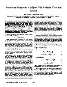
In applying IDM to a system of equations in which each equation corresponds to a particular frequency, the magnitudes of the diagonals of the IDM clearly indicate resonant regions. High values indicate near resonance. To illustrate, equation (4) is computed for a simple two degrees of freedom system and each single equation corresponds to one particular frequency covering the dynamic range of the system and the IDM is computed and its diagonals are used to weigh equations (4). The solid line of the top graph of Figure (1) shows the diagonals of the IDM as function of frequency. Comparing this to the transfer function in the bottom graph shows the correlation of the IDM to resonant regions. By inverse weighting of equations with the diagonals of IDM, the equations corresponding to resonant regions are underweighted as shown by the dashed line in the top graph. example on information density matrix and resonant frequencies

k,

k,

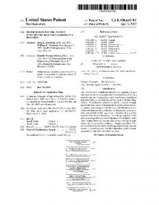
Figure 2. Symmetrrical Undamped Five DOF System

=

0.8

kt 3000 N/m, k2 m2 = 1.5 kg

?;-

·~ 0.6

~

.e.5 0.4 u

was selected to be undamped. A five degrees of freedom system was selected for investigation. The system is shown in Figure (2). The system's parameters shown on the figure are considered the exact , or the test, parameters. Measurements were selected at mass number 1, the left mass, and mass number 3 which is located at the node of mode two and close to the node of mode 4.

=45000 N/m, k3 =1000 N/m, m1 =1 kg,

initial

J

weighted

-----------

I

I

0o~----~0~.5------~~~----~~~.5~-----2~~L-~2.5 frequency (r/s)

10,-------.-------.-------.-------.------,

This system was used by Link [12]. Four analytical models are used for updating. Four parameters are assumed in error k1, k2, k3 and m 1; (in this example it is not possible to correct m2 since it has the exact same sensitivity as k2). Table 1. lists the ratios between analytical and test parameters. Figures 3.a and 3.b show the analysis and test transfer functions. Table 1: Stiffness and Mass Deviations of the Four Analytical Models

0 0~----~0~.5---====t====~--1.~5------~2~--~~2.5

frequency (r/s)

Figure 1. Application of Information Density Matrix to a 2-DOF System In implementing the IDM in this work, the diagonals of the IDM of equation (4) are used to calculate a diagonal matrix [W] where:

[W]

= (diagunal[D])wp

(11)

1.2 .85 .9 1.1 1.0

2 .95 .92 1.1 1.15 1.0

3 .85 1.15 1.1 .85 1.0

4 1.15 1.2 .8 .95 1.0

Several updating cases are performed with varying parameters and conditions to study: 1. Effect of selected frequencies,

where wp is a selected weighting power to accelerate the elimination of unstable frequency regions. To avoid numerical underflow a tolerance is applied such that: min (D)wp =tolerance

Model k1 k2 k3 m1 m2

2. Effects and selection of weighting power (wp in equation 11),

3. Effect of noise.

(12) 3.1 Choice of Weighting Power (wp)

3. APPLICATION AND PARAMETRIC STUDY In seeking an example to illustrate the applicability and validity of the proposed methods, it was important to have a system with relatively close resonances to minimize the available stable frequency region. In addition a symmetrical system was sought with one of the measurements being on the node of more than one mode. As well, since damping is known to increase the radius of convergence, the system

1070

According to equation (11), wp is dependent on the minimum value of the IDM and the chosen tolerance for a particular set of frequencies .To properly select the effective tolerance, and by tum wp, an initial noniterative study is conducted on the solution of equations (4) and (6) by varying the tolerance. The effect of the tolerance on: a) The condition number of the system of equations, b) Equations residuals,

frequencies, which are away from resonances, the noise to signal ratio is much higher.

c) Amount of change in correction parameters. Several cases are studied out of which some typical results are shown in Figures (4.1) and (4.2) for different frequency ranges as annotated on each figure. The three quantities a,b and c above are plotted versus the logarithm of the tolerance of equation (11).

The test is for frequency range 0 to 60 Hz and the transfer functions used are shown in Figures (8.1) and (8.2) while Figure (8.3) shows the updating results. It is observed that the technique converges to results bound by smaller errors than those in the data used.

These plots are important for the choice of the proper tolerance.They can even indicate that the chosen range of frequency is inappropriate for successful updating.

3.4 Convergence and Line Search Optimization

The choice of proper tolerance should be in regions of lower and flat condition number, lower and flat change in parameters and reasonable equations residuals; as illustrated in the next section.

In the iterative procedures implemented in this study to optimize the objective function, the line search method, [13], is used with some variation. Here , and at every iteration, the objective function is evaluated at end of step and at the middle point of the step. The point with the smaller objective function is taken. The line search is continued until the smallest objective function is found at this particular iteration. This may slow the convergence but helps against divergence.

3.2 Updating of Analytical Models All updatings are performed on the four analytical models. The test data is taken at measurements 1 and 3 with 41 frequency points at varying ranges.

4. CONCLUSIONS

Considering a pre-resonance range ofO to 20hz, Figure (4.1) indicates that the optimum tolerance is one or wp of zero. This is quite logical since there are no resonance frequencies in this range. Figure (5.1) shows the convergence of the correction parameters. A lower tolerance, which is equivalent to higher weighting power, does not help in this case. Figure (5.2) shows the updating results for a tolerance of 1Oe-4. Eventhough convergence is achieved, the condition number is needlessly higher as shown in Figure (5.3). Considering the frequency range of 0 to 40 hz which contains two resonance frequencies, Figure (4.2) suggests stable condition number for powers of less than -4. Figures (5.4) and (5.5) show updating results for powers of -6 and -9 respectively. Figure (5.6) shows the condition number for both cases. To illustrate the use and effects of the Information Density Matrix for this case, Figure (6) shows the diagonal for the IDM for the set of equations for the four analytical models. The IOM is again computed for the same equations weighted by the initial IDM. This dashed line clearly shows how the IDM is effective in removing the the unstable resonance frequencies. These results are shown for the15th iteration. Figure (7) shows the updating results when using one analytical model. This figure compares to the case in Figure 5.1

The use of Multi-Perturbed Analytical Model (MAM) combined with the use of the Information Density Matrix (I OM) is shown to be effective in updating af analytical models using measured Frequency Response Functions. The IDM information is used to weight the system of linear equations in such a way to eliminate the instability resulting from using data from the near resonances regions. The methods presented are shown to be computationally simple and poses numerical stability and well conditioned systems of equations. Thus as illustrated is insensitive to noisy data. 5. ACKNOWLEDGEMENT The first author participated in this work as a consultant to ESTEC in Summer 1997. He acknowledges the support of Dr. C. Stavrinidis and Mr. M. Klein. REFERENCES 1.

2.

3.3 Effects of Experimental Noise 3. Using the same updating example, the test transfer functions are corrupted with simulated experimental noise. The nose is uniformly distributed random signal with zero mean and variance of one. The amplitude of the noise is adjusted to be 2% of the maximum value of the FRF's. This is a considerably harsh amount of noise since at the usable

1071

4.

Lin, R. M. and Ewins, D. J., "Model Updating Using FRF Data," Proceedings of the Leuven 15th International Seminaron Modal Analysis; Belgium 1990; pp 141-162. Ibrahim, S.R., D'Ambrogio W.; Salvini, P. and Sestieri, A., "Direct Updating of Non-Conservative Finite Element Models Using Measured input-Output," SEM !MAC Proceedings; 1992; pp 202-210. Friswell, M. I. and Mottershead, J. E., "Model Updating in Structural Dynamics: A Survey," Journal of Sound and Vibration; 1993; 167; pp 347-375. Larsson, P. 0. Sas, P. , "Model Updating Based on Forced Vibrations Testing Using Numerically Stable Formulation," SEM IMAC 10 Proceedings; 1992; pp 996974.

5.

10. Powell, R. E., "Determining Source Signatures from Vibration Measurements and Transfer Functions," Proceedings of Noise-Con. 83, Cambridge, Massachusetts; 1983; pp 323-332.

Cogan, S.; Lenoir, D. and Lallement, G., "An Improved Frequency Response Residuals for Model Correction," SEM IMAC 14 Proceedings; February 1996; pp 568575. Teichert, W. and Schueller," "Convergence of Algorithms Using Frequency Response Data," ICOSSAR Proceedings, Japan; November 1997. Goyder, H. G. D., "Methods and Applications of Structural Modeling From Measured Structural Frequency Response Data," Journal of Sound and Vibrations (1980) 68(2); pp 209-228. Ibrahim, S. R.; Teichert, W. and Brunner, 0. , "Multi Perturbed Analytical Models for Updating and Damage Detection," SEM IMAC 15 proceedings; 1997; pp 127141. Jackson, D. D., "Interpretation of Inaccurate and Inconsistent Data," Geophisics Journal R. Astr. Soc.; (1972) 28; pp 97-109.

6.

7.

8.

9.

11. D'Ambrogio, W. and Fregolent, A., "On The Use of Consistent and Significant Information to Reduce IllConditioning in Dynamic Model Updating," Journal of Mechanical Systems and Signal Processing (In Press 1997). 12. Link, M., "Application of a Method for Identifying Incomplete System Matrices Using Vibration Test Data," Z. Flugwiss, Weltraumforsch. 9 (1985) Heft 3; pp 179-187. 13. Natke, H. G., Einfuhrung in Theorie und Praxis der Zeitreihen-und Modalanalyse, Friedr. Vieweg & Sohn; 1983. test and analysis frfs meas. 3 10-' ~-.,---.---.-=-:;:-=~:...::...:-.---r---r---r-l

test and analysis frfs meas. 1

10-'

.--r--.,---.---.--.:_,_--,----.---r---r----,

tes1

test 10-J

10...

II II I

\

',analysis

10...

\

\

\

\

\

I' II

10 ..

I 10-7 L__J.___ 0 10

_.___

_.___~_-:'--_--'-:-_-=----=----:::~---::

20

30

40 50 60 frequency (Hz)

(a)

70

80

90

10

100

_,

L _ 10_,___

0

0

_.___--'----"::----:::---:;;-.L7¢.:.0-~s;;';;o~-gg'iio~~1oo 20

30

40 50 6 frequency (Hz)

(b)

Figure 3. Test and Analysis Frequency Response Functions

i}: • ···~~~~~ ;:::f (I . :: :J (I :::

for frequenaes of 0 : 1 : 40 Hz

-~

~ 10' ' - - - - ' - - - - ' - - - - ' - - - - : ' - - - . . . . L_

-20

"'

-20

-18

-18

-16

-16

-14

-14

-12

-12

-10

-10

-8

-8

-6

-6

-4

-4

-2

-2

0

0

[I : : : : : : : : :l t'- -20

-18

-16

-14

-12 -10 -8 -6 power of tolerance; 101= 1o•x

(4.1)

-4

-2

0

-20

-18

-16

-14

"' -20

-18

-16

-14

t'- -20

-18

-16

-14

-12

-12

-10

-10

_ _ _ _ L _ - " . . _ - - - ' . _ - - ' ._ _

-8

-8

-6

-4

-2

0

: .\l

-6

-4

-2

0

-12 -10 -8 -6 power of tolerance; !01=1 o•x

-4

-2

0

j:~:r:: ~'i

Figure 4. Effects of Choice Tolerance on Updating Parameters

1072

~

10'r----------------

(4.2)

1·0:1 :40. tol=10e-6 1~:.5:20

; 101= 1

i .!!!

~ 1.05 0

c

I!! CD

Q;

E ~

~0.95

gu

0.9

0.85 0.8 0

10

5

0

15

10

15

iteration no.

iteration no.

(5.4)

(5.1) 1.4

1.3

1~:.5:20

i

~

; 1ol= 1Oe-4

~ 1.2 ii

1.05

~

1~0:1

:40. tol=10e-9

E 0 c

g

~1.1

.

e

~

~

a.

~ t::0.95

~

8

1

0.85 0.8 0

10

5

0.8 0

15

10

5

15

iteration no.

iteration no.

(5.5)

(5.2) 260

3000

--------

240

2500 I

I

220

1oi~10e-4

g

I

0

-ti 200

2000

c

I

0

-=

I

c

8

11500

X

~

E

-~

180

tOI=10e-9

1U E 1000

160 500

140

120 ---..__.....0

10

5

15

10

5

iteration no.

iteration no.

(5.3) Figure 5.

(5.6) Updating Results for Two Frequency Ranges with No Noise

1073

15

0.8 initial

0.7

1..0:1 :40, tol=1e-6 0.6 ONE MODEL

~

0.5

~ 1.05

·f