2016.10.27
Frequency Response with MATLAB Examples Control Design and Analysis Hans-Petter Halvorsen
PID Control
Hans-Petter Halvorsen, M.Sc.
Control System 𝑟
𝑒 −
Controller
Filtering
𝑢
Actuators
Sensors
𝑟 – Reference Value, SP (Set-point), SV (Set Value) 𝑦 – Measurement Value (MV), Process Value (PV) 𝑒 – Error between the reference value and the measurement value (𝑒 = 𝑟 – 𝑦) 𝑣 – Disturbance, makes it more complicated to control the process 𝑢 - Control Signal from the Controller
𝑣
Process
𝑦
The PID Algorithm 7
𝐾+ 3 𝑒𝑑𝜏 + 𝐾+ 𝑇. 𝑒̇ 𝑢 𝑡 = 𝐾+ 𝑒 + 𝑇- 8 Where 𝑢 is the controller output and 𝑒 is the control error:
𝑒 𝑡 = 𝑟 𝑡 − 𝑦(𝑡)
𝑟 is the Reference Signal or Set-point 𝑦 is the Process value, i.e., the Measured value
Tuning Parameters:
𝐾+ 𝑇𝑇.
Proportional Gain Integral Time [sec. ] Derivative Time [sec. ]
The PI Algorithm 7
𝐾+ 3 𝑒𝑑𝜏 𝑢 𝑡 = 𝐾+ 𝑒 + 𝑇- 8 Where 𝑢 is the controller output and 𝑒 is the control error:
𝑒 𝑡 = 𝑟 𝑡 − 𝑦(𝑡)
𝑟 is the Reference Signal or Set-point 𝑦 is the Process value, i.e., the Measured value
Tuning Parameters:
𝐾+ 𝑇-
Proportional Gain Integral Time [sec. ]
PI(D) Algorithm in MATLAB • Use pid() function in MATLAB • Define the PI(D) transfer function using the tf() function in MATLAB • We can also define and implement a discrete PI(D) algorithm
Discrete PI Controller Algorithm We start with: 𝑢 𝑡 = 𝑢8 + 𝐾+ 𝑒 𝑡 +
𝐾+ 7 3 𝑒𝑑𝜏 𝑇- 8
In order to make a discrete version using, e.g., Euler, we can derive both sides of the equation: 𝐾+ 𝑢̇ = 𝑢̇ 8 + 𝐾+ 𝑒̇ + 𝑒 𝑇If we use Euler Forward we get: 𝑢? − 𝑢?@A 𝑢8,? − 𝑢8,?@A 𝑒? − 𝑒?@A 𝐾+ = + 𝐾+ + 𝑒 𝑇B 𝑇B 𝑇B 𝑇- ? Then we get: 𝐾+ 𝑢? = 𝑢?@A + 𝑢8,? − 𝑢8,?@A + 𝐾+ 𝑒? − 𝑒?@A + 𝑇𝑒 𝑇- B ? Where
𝑒? = 𝑟? − 𝑦? We can also split the equation above in 2 different parts by setting: ∆𝑢? = 𝑢? − 𝑢?@A This gives the following PI control algorithm: 𝑒? = 𝑟? − 𝑦? ∆𝑢? = 𝑢8,? − 𝑢8,?@A + 𝐾+ 𝑒? − 𝑒?@A + 𝑢? = 𝑢?@A + ∆𝑢? This algorithm can easily be implemented in MATLAB
𝐾+ 𝑇𝑒 𝑇- B ?
Discrete PI Controller Algorithm Discrete PI control algorithm:
𝑒? = 𝑟? − 𝑦? ∆𝑢? = 𝑢8,? − 𝑢8,?@A + 𝐾+ 𝑒? − 𝑒?@A 𝑢? = 𝑢?@A + ∆𝑢?
𝐾+ + 𝑇B 𝑒? 𝑇-
PID Controller –Transfer Function We have:
𝐾+ 7 3 𝑒𝑑𝜏 + 𝐾+ 𝑇. 𝑒̇ 𝑢 𝑡 = 𝐾+ 𝑒 + 𝑇- 8
Laplace gives:
𝐻FGH
𝐾+ 𝑢(𝑠) 𝑠 = = 𝐾+ + + 𝐾+ 𝑇. 𝑠 𝑒(𝑠) 𝑇- 𝑠
𝐻FGH
𝑢(𝑠) 𝐾+ (𝑇. 𝑇- 𝑠 J + 𝑇- 𝑠 + 1) 𝑠 = = 𝑒(𝑠) 𝑇- 𝑠
or:
PI Controller –Transfer Function We have:
𝐾+ 7 3 𝑒𝑑𝜏 𝑢 𝑡 = 𝐾+ 𝑒 + 𝑇- 8
Laplace gives:
𝐻FG
𝐾+ 𝐾+ 𝑇- 𝑠 + 𝐾+ 𝐾+ (𝑇- 𝑠 + 1) 𝑢(𝑠) 𝑠 = = 𝐾+ + = = 𝑒(𝑠) 𝑇- 𝑠 𝑇- 𝑠 𝑇- 𝑠
Finally:
𝐻FG
𝑢(𝑠) 𝐾+ (𝑇- 𝑠 + 1) 𝑠 = = 𝑒(𝑠) 𝑇- 𝑠
Define PI Transfer function in MATLAB clear, clc
𝐻FG
𝑢(𝑠) 𝐾+ (𝑇- 𝑠 + 1) 𝑠 = = 𝑒(𝑠) 𝑇- 𝑠
% PI Controller Transfer function Kp = 0.52; Ti = 18; num = Kp*[Ti, 1]; den = [Ti, 0]; Hpi = tf(num,den) ...
PI Controller – State space model Given: A
𝐾+ 𝑢 𝑠 = 𝐾+ 𝑒 𝑠 + 𝑒 𝑠 𝑇- 𝑠
We set 𝑧 = 𝑒 ⇒ 𝑠𝑧 = 𝑒 ⇒ 𝑧̇ = 𝑒 B This gives: 𝑧̇ = 𝑒
Where
𝐾+ 𝑢 = 𝐾+ 𝑒 + 𝑧 𝑇𝑒 =𝑟−𝑦
PI Controller – Discrete State space model Using Euler: 𝑧̇ ≈ Where 𝑇B is the Sampling Time. This gives:
Finally:
𝑧?OA − 𝑧? 𝑇B
𝑧?OA − 𝑧? = 𝑒? 𝑇B 𝐾+ 𝑢? = 𝐾+ 𝑒? + 𝑧 𝑇- ? 𝑒? = 𝑟? − 𝑦? 𝐾+ 𝑢? = 𝐾+ 𝑒? + 𝑧 𝑇- ? 𝑧?OA = 𝑧? + 𝑇B 𝑒?
PI Controller – Discrete State space model implemented in MATLAB clear, clc ... for i=1:N ... e = r - y; u = Kp*e + z; z = z + dt*Kp*e/Ti; ... end plot(...)
Frequency Response Hans-Petter Halvorsen, M.Sc.
Frequency Response
Theory
• The frequency response of a system is a frequency dependent function which expresses how a sinusoidal signal of a given frequency on the system input is transferred through the system. Each frequency component is a sinusoidal signal having certain amplitude and a certain frequency. • The frequency response is an important tool for analysis and design of signal filters and for analysis and design of control systems. • The frequency response can be found experimentally or from a transfer function model. • The frequency response of a system is defined as the steady-state response of the system to a sinusoidal input signal. When the system is in steady-state, it differs from the input signal only in amplitude/gain (A) and phase lag (𝜙).
Theory
Frequency Response
Input Signal
𝑢 𝑡 = 𝑈 R 𝑠𝑖𝑛𝜔𝑡 Amplitude
Input Signal
Dynamic System
Output Signal
Output Signal
𝑦 𝑡 = 𝑈𝐴 W 𝑠𝑖𝑛(𝜔𝑡 + 𝜙) X
Frequency Gain
Phase Lag
The frequency response of a system expresses how a sinusoidal signal of a given frequency on the system input is transferred through the system. The only difference is the gain and the phase lag.
Frequency Response - Definition 𝑦 𝑡 = 𝑈𝐴 W 𝑠𝑖𝑛(𝜔𝑡 + 𝜙)
𝑢 𝑡 = 𝑈 R 𝑠𝑖𝑛𝜔𝑡
X
Input
Dynamic System
𝜔 = 1 𝑟𝑎𝑑/𝑠 and the same for Frequency 2, 3, 4, 5, 6, etc. • •
Theory
Output
𝜔 = 1 𝑟𝑎𝑑/𝑠
The frequency response of a system is defined as the steady-state response of the system to a sinusoidal input signal. When the system is in steady-state, it differs from the input signal only in amplitude/gain (A) (Norwegian: “forsterkning”) and phase lag (ϕ) (Norwegian: “faseforskyvning”).
Frequency Response Simple Example
Theory
Outside Temperature
T = 1 year
frequency 1 (year)
Dynamic System Inside Temperature
frequency 1 (year)
Note! Only the gain and phase are different
Assume the outdoor temperature is varying like a sine function during a year (frequency 1) or during 24 hours (frequency 2). Then the indoor temperature will be a sine as well, but with different gain. In addition it will have a phase lag.
Frequency Response Simple Example
Theory
Outside Temperature T = 24 hours
frequency 2 (24 hours)
Dynamic System Inside Temperature
frequency 2 (24 hours)
Note! Only the gain and phase are different
Assume the outdoor temperature is varying like a sine function during a year (frequency 1) or during 24 hours (frequency 2). Then the indoor temperature will be a sine as well, but with different gain. In addition it will have a phase lag.
Frequency response using Bode Diagram Hans-Petter Halvorsen, M.Sc.
Bode Diagram You can find the Bode diagram from experiments on the physical process or from the transfer function (the model of the system). A simple sketch of the Bode diagram for a given system:
𝜔𝑐
0𝑑𝐵
∆𝐾
𝐿𝑜𝑔 𝜔
ω [rad/s]
The Bode diagram gives a simple Graphical overview of the Frequency Response for a given system. A Tool for Analyzing the Stability properties of the Control System. With MATLAB you can easily create Bode diagram from the Transfer function model using the bode() function
𝜑
𝜔180
𝐿𝑜𝑔 𝜔
ω [rad/s]
Bode Diagram from experiments Find Data for different frequencies
...
Based on that we can plot the Frequency Response in a so-called Bode Diagram:
We find 𝐴 and 𝜙 for each of the frequencies, e.g.:
Bode Diagram
The x-scale is logarithmic
Gain (“Forsterkningen”) Note! The y-scale is in [𝑑𝐵]
𝑥 𝑑𝐵 = 20𝑙𝑜𝑔A8 𝑥
Phase lag (“Faseforkyvningen”) The y-scale is in [𝑑𝑒𝑔𝑟𝑒𝑒𝑠]
2𝜋 𝑟𝑎𝑑 = 360°
Normally, the unit for frequency is Hertz [Hz], but in frequency response and Bode diagrams we use radians ω [rad/s]. The relationship between these are as follows:
𝜔 = 2𝜋𝑓
Frequency Response – MATLAB Transfer Function:
MATLAB Code: clear clc close all % Define Transfer function num=[1]; den=[1, 1]; H = tf(num, den) % Frequency Response bode(H); grid on
The frequency response is an important tool for analysis and design of signal filters and for analysis and design of control systems.
Frequency Response – MATLAB
Transfer Function:
clear clc close all
Instead of Plotting the Bode Diagram we can also use the bode function for calculation and showing the data as well: freq_data = 0.0100 0.1000 1.0000 2.0000 3.0000 5.0000 10.0000 100.0000
-0.0004 -0.0432 -3.0103 -6.9897 -10.0000 -14.1497 -20.0432 -40.0004
-0.5729 -5.7106 -45.0000 -63.4349 -71.5651 -78.6901 -84.2894 -89.4271
% Define Transfer function num=[1]; den=[1, 1]; H = tf(num, den) % Frequency Response bode(H); grid on % Get Freqquency Response Data wlist = [0.01, 0.1, 1, 2 ,3 ,5 ,10, 100]; [mag, phase, w] = bode(H, wlist); for i=1:length(w) magw(i) = mag(1,1,i); phasew(i) = phase(1,1,i); end magdB = 20*log10(magw); % Convert to dB freq_data = [wlist; magdB; phasew]'
Bode Diagram – MATLAB Example MATLAB Code: clear, clc % Transfer function num=[1]; den1=[1,0]; den2=[1,1] den3=[1,1] den = conv(den1,conv(den2,den3)); H = tf(num, den) clear, clc
% Bode Diagram bode(H) subplot(2,1,1) grid on subplot(2,1,2) grid on
% Transfer function num=[1]; den=[1,2,1,0]; H = tf(num, den)
or:
% Bode Diagram bode(H) subplot(2,1,1) grid on subplot(2,1,2) grid on
Example We will use the following system as an example:
1 𝐻+ = 𝑠(𝑠 + 1)
𝐻k = 𝐾+ 𝑟
𝑒 −
Controller
𝑢
Sensors
1 𝐻l = 3𝑠 + 1
Process
𝑦
Bode Diagram – MATLAB Example MATLAB Code: clear clc num = 1; den = [1,1,0]; Hp = tf(num,den) bode(Hp) grid on
1 𝐻+ = 𝑠(𝑠 + 1)
Complex Numbers Background Theory for Frequency Response
Hans-Petter Halvorsen, M.Sc.
Complex Numbers A Complex Number is given by:
𝑧 = 𝑎 + 𝑗𝑏
Where 𝑗 = −1 We have that:
𝐼𝑚𝑎𝑔𝑖𝑛𝑎𝑟𝑦 𝐴𝑥𝑖𝑠 (𝐼𝑚)
𝑎 = 𝑅𝑒 𝑧 𝑏 = 𝐼𝑚(𝑧)
𝑧 = 𝑎 + 𝑗𝑏
𝑏
0
𝑎
𝑅𝑒𝑎𝑙 𝐴𝑥𝑖𝑠(𝑅𝑒)
Complex Numbers Polar form:
𝑗 = −1
𝑧 = 𝑟𝑒 st
Where: 𝑎J +𝑏 J 𝑏 𝜃 = 𝑎𝑡𝑎𝑛 𝑎
𝑟= 𝑧 =
Note! 𝑎 = 𝑟 cos 𝜃
𝐼𝑚𝑎𝑔𝑖𝑛𝑎𝑟𝑦 𝐴𝑥𝑖𝑠 (𝐼𝑚)
𝑧 = 𝑟𝑒 st
𝑏 𝑟
𝑏 = 𝑟 sin 𝜃 0
𝜃 𝑎
𝑅𝑒𝑎𝑙 𝐴𝑥𝑖𝑠(𝑅𝑒)
Complex Numbers 1
Rectangular form of a complex number 𝐼𝑚𝑎𝑔𝑖𝑛𝑎𝑟𝑦 𝐴𝑥𝑖𝑠 (𝐼𝑚)
2
Exponential/polar form of a complex number 𝐼𝑚𝑎𝑔𝑖𝑛𝑎𝑟𝑦 𝐴𝑥𝑖𝑠 (𝐼𝑚)
𝑧 = 𝑎 + 𝑗𝑏
𝑏
𝑧 = 𝑟𝑒 st
𝑏 𝑟
0
𝑎
𝑅𝑒𝑎𝑙 𝐴𝑥𝑖𝑠(𝑅𝑒)
Length (“Gain”):
𝑟 = 𝑧 =
𝑗 = −1
𝜃
0
Angle (“Phase”):
𝑎J + 𝑏 J
𝑎
𝑅𝑒𝑎𝑙 𝐴𝑥𝑖𝑠(𝑅𝑒)
𝑏 𝜃 = 𝑎𝑡𝑎𝑛 𝑎
Frequency response from Transfer function Hans-Petter Halvorsen, M.Sc.
Manually find the Frequency Response from the Transfer Function For a transfer function: 𝐻 𝑆 =
𝑦(𝑠) 𝑢(𝑠)
We have that:
Theory
𝑠 = 𝑗𝜔
𝐻 𝑗𝜔 = 𝐻(𝑗𝜔) 𝑒 s∠{(s|) Where 𝐻(𝑗𝜔) is the frequency response of the system, i.e., we may find the frequency response by setting 𝑠 = 𝑗𝜔 in the transfer function. Bode diagrams are useful in frequency response analysis. The Bode diagram consists of 2 diagrams, the Bode magnitude diagram, 𝐴(𝜔) and the Bode phase diagram, 𝜙(𝜔). The Gain function: 𝐴 𝜔 = 𝐻(𝑗𝜔) The Phase function: 𝜙 𝜔 = ∠𝐻(𝑗𝜔) The 𝐴(𝜔)-axis is in decibel (dB), where the decibel value of x is calculated as: 𝑥 𝑑𝐵 = 20𝑙𝑜𝑔A8 𝑥 The 𝜙(𝜔)-axis is in degrees (not radians!)
Mathematical expressions for 𝐴(𝜔) and 𝜙(𝜔) We find the Mathematical expressions for 𝐴(𝜔) and 𝜙(𝜔) by setting 𝑠 = 𝑗𝜔 in the transfer function given by: 𝑦(𝑠) 𝐾 𝐻 𝑠 = = 𝑢(𝑠) 𝑇𝑠 + 1 The Frequency Response (we replace 𝑠 with 𝑗𝜔) then becomes: 𝐾 𝐾 𝐻 𝑗𝜔 = = 𝑇𝑗𝜔 + 1 ⏟ 1 + 𝑗 𝑇𝜔 W ~•
Polar form:
𝐾
𝐻 𝑗𝜔 = =
𝐾
1J + 𝑇𝜔 J 𝑒
1 + 𝑇𝜔
Finally: 𝐻 𝑗𝜔 =
Gl
J
s €•k7€‚
ƒ| A
𝑒 s @€•k7€‚(ƒ|)
𝐾 1 + 𝑇𝜔
J
𝑒 s @€•k7€‚(ƒ|) cont. next page
cont. from previous page
The Gain function becomes: 𝐴 𝜔 = 𝐻(𝑗𝜔) =
𝐾 1 + 𝑇𝜔
J
Or in 𝑑𝐵 (used in the Bode Plot): 𝐴 𝜔 .„ = 𝐻(𝑗𝜔) .„ = 20𝑙𝑜𝑔𝐾 − 20𝑙𝑜𝑔 1 + 𝑇𝜔
J
The Phase function becomes ( 𝑟𝑎𝑑 ): 𝜙 𝜔 = ∠𝐻 𝑗𝜔 = 𝑎𝑟𝑔 𝐻 𝑗𝜔 = −𝑎𝑟𝑐𝑡𝑎𝑛(𝑇𝜔) Or in degrees ° (used in the Bode plot): 𝜙 𝜔 = ∠𝐻 𝑗𝜔 = −𝑎𝑟𝑐𝑡𝑎𝑛(𝑇𝜔) R
180 𝜋
Note: 2𝜋 𝑟𝑎𝑑 = 360°
Transfer function:
𝑨(𝝎) og 𝝓(𝝎):
1 𝐻 𝑠 = 𝑠+1 4 𝐻 𝑠 = 2𝑠 + 1
𝐻(𝑗𝜔)
𝐻(𝑗𝜔)
.„
= 20𝑙𝑜𝑔4 − 20𝑙𝑜𝑔 (2𝜔)J +1
∠𝐻(𝑗𝜔) = −arctan(2𝜔) 𝐻(𝑗𝜔)
.„
= 20𝑙𝑜𝑔5 − 20𝑙𝑜𝑔 (𝜔)J +1 − 20𝑙𝑜𝑔 (10𝜔)J +1 ∠𝐻(𝑗𝜔) = −arctan(𝜔) − arctan(10𝜔)
𝐻(𝑗𝜔)
= −20𝑙𝑜𝑔 (𝜔)J − 2𝑥20𝑙𝑜𝑔 (𝜔)J +1
= 20𝑙𝑜𝑔𝜔 − 40𝑙𝑜𝑔 (𝜔)J +1
J
∠𝐻(𝑗𝜔) = −90 − 2 arctan (𝜔)
3.2𝑒 @JB 𝐻 𝑠 = 3𝑠 + 1
𝐻(𝑗𝜔)
.„
= 20𝑙𝑜𝑔3.2 − 20𝑙𝑜𝑔 (3𝜔)J +1
∠𝐻(𝑗𝜔) = −2𝜔 − arctan(3𝜔) 𝐻(𝑗𝜔)
.„
= 20𝑙𝑜𝑔 (5𝜔)J +1 − 20𝑙𝑜𝑔 (2𝜔)J +1 − 20𝑙𝑜𝑔 (10𝜔)J +1
∠𝐻(𝑗𝜔) = arctan(5𝜔) − arctan(2𝜔) − arctan(10𝜔)
•
5𝑠 + 1 𝐻 𝑆 = 2𝑠 + 1 (10𝑠 + 1)
.„
Note! In order to find the phase in A•8 degrees, we have to multiply with:
1 𝑠 𝑠+1
= 20𝑙𝑜𝑔1 − 20𝑙𝑜𝑔 (𝜔)J +1
∠𝐻(𝑗𝜔) = −arctan(𝜔)
5 𝐻 𝑆 = 𝑠 + 1 (10𝑠 + 1) 𝐻 𝑆 =
.„
Manually find the Frequency Response from the Transfer Function Given the following transfer function: 4 𝐻 𝑆 = 2𝑠 + 1
Bode Plot:
The mathematical expressions for 𝐴(𝜔) and 𝜙(𝜔) become: 𝐻(𝑗𝜔)
.„
= 20𝑙𝑜𝑔4 − 20𝑙𝑜𝑔 (2𝜔)J +1
∠𝐻(𝑗𝜔) = −arctan(2𝜔) These equations can easily be implemented in MATLAB (See next slide)
clear clc % Transfer function num=[4]; den=[2, 1]; H = tf(num, den) % Bode Plot figure(1) bode(H) grid on % Margins and Phases for given Frequencies % Alt 1: Use bode function directly disp('----- Alternative 1 -----') w = [0.1, 0.16, 0.25, 0.4, 0.625, 2.5, 10]; [magw, phasew] = bode(H, w); for i=1:length(w) mag(i) = magw(1,1,i); phase(i) = phasew(1,1,i); end magdB = 20*log10(mag); %convert to dB mag_data = [w; magdB] phase_data = [w; phase]
MATLAB Code clear clc w = [0.1, 0.16, 0.25, 0.4, 0.625, 2.5, 10]; % Alt 2: Use Mathematical expressions for H and
Solutions
From the Bode diagram we can verify that our calculations are correct:
𝐴 = −3.35 𝑑𝐵
𝜙 = −45.9 °
𝜔 = 1 rad/s
The following MATLAB Code is used to create the Plot: clear, clc K = T = num den H =
1; 1; = [K]; = [T, 1]; tf(num, den);
figure(1) bode(H), grid on % Define input signal t = [1: 0.1 : 12]; w = 1; U = 1; u = U*sin(w*t); figure(2) plot(t, u) % Output signal hold on lsim(H, ':r', u, t) grid on hold off legend('input signal', 'output signal')
We use the following transfer function: 𝐻 𝑠 =
1 𝑠+1
The Frequency used: 𝜔 = 1 rad/s
PID Controller Design/Tuning Hans-Petter Halvorsen, M.Sc.
PID Controller Design A lot of PID Tuning methods exist, e.g., • Skogestad's method • Ziegler-Nichols’ methods • Trial and Error Methods • PID Tuning functionality built into MATLAB • Auto-tuning built into commercial PID controllers • ...
Skogestad’s method • The Skogestad’s method assumes you apply a step on the input (𝑢) and then observe the response and the output (𝑦), as shown below. • If we have a model of the system (which we have in our case), we can use the following Skogestad’s formulas for finding the PI(D) parameters directly.
𝑇k is the time-constant of the control system which the user must specify
Figure: F. Haugen, Advanced Dynamics and Control: TechTeach, 2010.
Originally, Skogestad defined the factor 𝑐 = 4. This gives good set-point tracking. But the disturbance compensation may become quite sluggish. To obtain faster disturbance compensation, you can use 𝑐 = 1.5
Ziegler–Nichols Frequency Response method Theory Assume you use a P controller only 𝑇- = ∞, 𝑇. = 0. Then you need to find for which 𝐾+ the closed loop system is a marginally stable system (𝜔k = 𝜔A•8 ). This 𝐾+ is called 𝐾k (critical gain). The 𝑇k (critical period) can be found from the damped oscillations of the closed loop system. Then calculate the PI(D) parameters using the formulas below. Marginally stable system: Controller 𝐾+ 𝑇𝑇. 𝜔k = 𝜔A•8 P 0.5𝐾k ∞ 0 𝑇k PI 0.45𝐾k 0 1.2 2𝜋 𝑇k 𝑇k 𝑇k = PID 0.6𝐾k 𝜔A•8 𝑇k 8 2
𝐾k - Critical Gain 𝑇k - Critical Period
https://en.wikipedia.org/wiki/Ziegler–Nichols_method
Controller Design/Tuning using MATLAB Hans-Petter Halvorsen, M.Sc.
Controller Design/Tuning using MATLAB • • • •
Frequency Design and Analysis pidtune() MATLAB function PID Tuner (Interactive Tools) ...
Validate with simulations!
pidtune() MATLAB function clear, clc %Define Process num = 1; den = [1,1,0]; Hp = tf(num,den) % Find PI Controller [Hpi,info] = pidtune(Hp,'PI') %Bode Plots figure(1) bode(Hp) grid on figure(2) bode(Hpi) grid on % Feedback System T = feedback(Hpi*Hp, 1); figure(3) step(T)
𝐾+ = 0.33 𝑇- =
1 1 = ≈ 43.5𝑠 𝐾- 0.023
pidtune() MATLAB function
To improve the response time, you can set a higher target crossover frequency than the result that pidtune() automatically selects, 0.32. Increase the crossover frequency to 1.0.
[Hpi,info] = pidtune(Hp,'PI', 1.0)
The new controller achieves the higher crossover frequency, but at the cost of a reduced phase margin.
MATLAB PID Tuner Define Controller Type
Tuning
Define your Process Add Additional Plots Step Response and other Plots can be shown
PID Parameters
Stability Analysis using MATLAB Hans-Petter Halvorsen, M.Sc.
Stability Analysis How do we figure out that the Feedback System is stable before we test it on the real System? 1. Poles 2. Frequency Response/Bode 3. Simulations (Step Response) We will do all these things using MATLAB
3 Time domain Asymptotically stable system
Stability Analysis 2 Frequency domain
lim 𝑦 𝑡 = 𝑘
7→š Tracking transfer function
Loop transfer function
Marginally stable system
Unstable system
1 The Complex domain
Poles
Tracking transfer function Figure: F. Haugen, Advanced Dynamics and Control: TechTeach, 2010.
Asymptotically stable system: 𝜔k < 𝜔A•8 Marginally stable system: 𝜔k = 𝜔A•8 Unstable system: 𝜔k > 𝜔A•8
Poles
1 Asymptotically stable system:
Each of the poles of the transfer function lies strictly in the left half plane (has strictly negative real part). 3 Unstable system: 2 Marginally stable system:
One or more poles lies on the imaginary axis (have real part equal to zero), and all these poles are distinct. Besides, no poles lie in the right half plane.
At least one pole lies in the right half plane (has real part greater than zero).
Or: There are multiple and coincident poles on the imaginary axis. A Example: double integrator 𝐻(𝑠) = œ B
Theory
Stability Analysis Asymptotically stable system:
Marginally stable system:
Unstable system:
lim 𝑦 𝑡 = ∞
lim 𝑦 𝑡 = 𝑘
7→š
7→š
Figures: F. Haugen, Advanced Dynamics and Control: TechTeach, 2010.
0 < lim 𝑦 𝑡 < ∞ 7→š
At least one pole lies in the right half plane (has real part greater than zero). Each of the poles of the transfer function lies strictly in the left half plane (has strictly negative real part).
One or more poles lies on the imaginary axis (have real part equal to zero), and all these poles are distinct. Besides, no poles lie in the right half plane.
Or: There are multiple and coincident poles on the imaginary axis. Example: double A integrator 𝐻(𝑠) = œ B
Stability Analysis of Feedback Systems Hans-Petter Halvorsen, M.Sc.
Stability Analysis of Feedback Systems
1
Loop Transfer Function (“Sløyfetransferfunksjonen”):
Hr = ... Hp = ... Hm = ... L = series(series(Hr, Hp), Hm)
2
The Tracking Function (“Følgeforholdet”): L = ... T = feedback(L, 1)
3
The Sensitivity Function (“Sensitivitetsfunksjonen”): T = ... S = 1-T
Theory
Frequency Response and Stability Analysis Bode Diagram
Theory
𝜔k and 𝜔A•8 are called the crossover-frequencies (“kryssfrekvens”)
Δ𝐾 is the gain margin (GM) of the system (“Forsterkningsmargin”). How much the loop gain can increase before the system becomes unstable
𝜙 is the phase margin (PM) of the system (“Fasemargin”). How much phase shift the system can tolerate before it becomes unstable.
Asymptotically stable system: 𝜔k < 𝜔A•8 Marginally stable system: 𝜔k = 𝜔A•8 Unstable system: 𝜔k > 𝜔A•8
Frequency Response and Stability Analysis
Theory
The definitions are as follows: Gain Crossover-frequency - 𝜔k : 𝐿 𝑗𝜔k
= 1 = 0𝑑𝐵
Phase Crossover-frequency - 𝜔A•8 : ∠𝐿 𝑗𝜔A•8 = −180
•
Gain Margin - GM (𝛥𝐾): 𝐺𝑀 𝑑𝐵 = − 𝐿 𝑗𝜔A•8 𝑑𝐵 Phase margin PM (𝜑): 𝑃𝑀 = 180• + ∠𝐿(𝑗𝜔k )
𝜔A•8 is the gain margin frequency, in radians/second. A gain margin frequency indicates where the model phase crosses -180 degrees. GM (Δ𝐾) is the gain margin of the system. 𝜔k is phase margin frequency, in radians/second. A phase margin frequency indicates where the model magnitude crosses 0 decibels. PM (𝜑) is the phase margin of the system.
We have that: 1. Asymptotically stable system: 𝜔k < 𝜔A•8 2. Marginally stable system: 𝜔k = 𝜔A•8 3. Unstable system: 𝜔k > 𝜔A•8
Stability Analysis of Feedback System - Example Hans-Petter Halvorsen, M.Sc.
Example We will use the following system as an example:
𝐻k = 𝐾+ 𝑟
𝑒 −
Controller
𝑢
Sensors
1 𝐻l = 3𝑠 + 1
1 𝐻+ = 𝑠(𝑠 + 1) Process
𝑦
Analysis of the Feedback System Loop transfer function: 𝑳(𝒔) We need to find the Loop transfer function 𝐿(𝑠) using MATLAB. The Loop transfer function is defined as:
𝐿 𝑠 = 𝐻k 𝐻+
We will use the built-in function series() in MATLAB.
Tracking transfer function: 𝑻(𝒔) We need to find the Tracking transfer function 𝑇(𝑠) using MATLAB. The Tracking transfer function is defined as:
𝑇 𝑠 =
¥(B) •(B)
=
¦(B) AO¦(B)
We will use the built-in function feedback() in MATLAB.
Sensitivity transfer function: 𝑺(𝒔) We need to find the Sensitivity transfer function 𝑆(𝑠) using MATLAB. The Sensitivity transfer function is defined as:
𝑆 𝑠 =
•(B) •(B)
=
A AO¦(B)
= 1 − 𝑇(𝑠)
Stability Analysis • Plot the Bode plot for the system using e.g., the bode() function in MATLAB • Find the crossover-frequencies (𝜔A•8 , 𝜔k ) and stability margins GM (𝐴(𝜔)), PM (𝜙(𝜔)) of the system (𝐿(𝑠)) from the Bode plot. • Plot also Bode diagram where the crossover-frequencies, GM and PM are illustrated. Tip! Use the margin() function in MATLAB. • Use also the margin() function in order to find values for 𝜔A•8 , 𝜔k , 𝐴(𝜔), 𝜙(𝜔) directly. • You should compare and discuss the results. • How much can you increase 𝐾+ before the system becomes unstable?
MATLAB Code:
clear, clc, clf
bode(L)
% The Process Transfer function Hp(s) num_p=[1]; den1=[1, 0]; den2=[1, 1]; den_p = conv(den1,den2); Hp = tf(num_p, den_p) % The Measurement Transfer function Hm(s) num_m=[1]; den_m=[3, 1]; Hm = tf(num_m, den_m)
margin(L)
% The Controller Transfer function Hr(s) Kp = 0.35; Hr = tf(Kp) % The Loop Transfer function L = series(series(Hr, Hp), Hm) % Bode Diagram figure(1) bode(L),grid on figure(2) margin(L) [gm, pm, w180, wc] = margin(L); wc w180 gm gmdB = 20*log10(gm) pm
wc w180 gm gmdB pm
= = = = =
0.2649 rad/s 0.5774 rad/s 3.8095 11.6174 dB 36.6917 degrees
From the Bode plot we can get: ∆𝐾 = 11.6 𝑑𝐵
𝜔k = 0.26 𝜙 = 37 ° 0.1
0.3 0.2
𝜔A•8 = 0.58 1 0.5
10
Stable vs. Unstable System • We will find and use different values of 𝐾+ where we get a marginally stable system, an asymptotically stable system and an unstable system. • We will Plot the time response for the tracking function using the step() function in MATLAB for all these 3 categories. How can we use the step response to determine the stability of the system? • We will find 𝜔A•8 , 𝜔k , 𝐴 𝜔 and 𝜙(𝜔) in all 3 cases. We will see how we use 𝜔k and 𝜔A•8 to determine the stability of the system. • We will find and plot the poles and zeros for the system for all the 3 categories mentioned above. We will see how we can we use the poles to determine the stability of the system. • Bandwidth: We will plot the Loop transfer function 𝐿(𝑠), the Tracking transfer function 𝑇(𝑠) and the Sensitivity transfer function 𝑆(𝑠) in a Bode diagram for the system for all the 3 categories mentioned above.
Stable System
𝐾+ = 0.35
For what 𝐾+ becomes the system marginally stable? 𝐾+l = 0.35 × Δ𝐾 = 0.35 × 3.8 ≈ 1,32
𝜔k < 𝜔A•8
wc w180 gm gmdB pm
lim 𝑦 𝑡 = 1
7→š
= = = = =
0.2649 rad/s 0.5774 rad/s 3.8095 11.6174 dB 36.6917 degrees Poles in the left half plane
Marginally Stable System 𝐾+ = 1.32 𝜔k = 𝜔A•8
0 < lim 𝑦 𝑡 < ∞ 7→š
wc w180 gm gmdB pm
= = = = =
0.5744 0.5774 1.0101 0.0873 0.2500
rad/s rad/s dB degrees
Poles at the imaginary axis
Unstable System 𝐾+ = 2 𝜔k > 𝜔A•8
lim 𝑦 𝑡 = ∞
7→š
wc w180 gm gmdB pm
= 0.7020 = 0.5774 = 0.6667 = -3.5218 = -9.6664
Poles in the right half plane
MATLAB Code clear, clc, clf % The Process Transfer function Hp(s) num_p=[1]; den1=[1, 0]; den2=[1, 1]; den_p = conv(den1,den2); Hp = tf(num_p, den_p) % The Measurement Transfer function Hm(s) num_m=[1]; den_m=[3, 1]; Hm = tf(num_m, den_m) % The Controller Transfer function Hr(s) Kp = 0.35; % Stable System %Kp = 1.32; % Marginally Stable System %Kp = 2; % Unstable System Hr = tf(Kp) % The Loop Transfer function L = series(series(Hr, Hp), Hm) % Tracking transfer function T=feedback(L,1); % Sensitivity transfer function S=1-T; ...
... % Bode Diagram figure(1) bode(L), grid on figure(2) margin(L), grid on [gm, pm, w180, wc] = margin(L); wc w180 gm gmdB = 20*log10(gm) pm % Simulating step response for control system (tracking transfer function) figure(3) step(T) % Poles pole(T) figure(4) pzmap(T) % Bandwidth figure(5) bodemag(L,T,S), grid on
“Golden rules” of Stability Margins for a Control System
Theory
Reference: F. Haugen, Advanced Dynamics and Control: TechTeach, 2010.
Gain Margin (GM): (Norwegian: “Forsterkningsmargin”)
Phase Margin (PM): (Norwegian: “Fasemargin”)
The Bandwidth of the Control System Hans-Petter Halvorsen, M.Sc.
The Bandwidth of the Control System • You should plot the Loop transfer function 𝐿(𝑠), the Tracking transfer function 𝑇(𝑠) and the Sensitivity transfer function 𝑆(𝑠) in the same Bode diagram. • Use, e.g., the bodemag() function in MATLAB (only the gain diagram is of interest in this case, not the phase diagram). • Use the values for 𝐾+ and 𝑇- found in a previous Tasks. • You need to find the different bandwidths 𝝎𝒕 , 𝝎𝒄 , 𝝎𝒔 (see the sketch below).
The Bandwidth of the Control System
Theory
The bandwidth of a control system is the frequency which divides the frequency range of good tracking and poor tracking. 3 different Bandwidth definitions:
𝐿 𝑇 𝑆
Good Tracking
Poor Tracking BW
Good Set-point Tracking: |𝑆(𝑗𝜔)| ≪ 1, |𝑇 (𝑗𝜔)| ≈ 1, |𝐿(𝑗𝜔)| ≫ 1
𝐾+ = 0.35
Good Set-point Tracking: |𝑆(𝑗𝜔)| ≪ 1, |𝑇 (𝑗𝜔)| ≈ 1, |𝐿(𝑗𝜔)| ≫ 1
𝐿 𝑇
𝑆 𝜔B = 0.092 0.05
0.1
𝜔k = 0.27 0.2
0.3
𝜔7 = 0.46 1
PI Controller Example Hans-Petter Halvorsen, M.Sc.
PI Controller - Example We will use the following system as an example:
𝐾+ (𝑇- 𝑠 + 1) 𝐻k = 𝑇- 𝑠
𝑟
𝑒 −
Controller
𝑢
Sensors
1 𝐻l = 3𝑠 + 1
1 𝐻+ = 𝑠(𝑠 + 1) Process
𝑦
Ziegler–Nichols Frequency Response method Theory Assume you use a P controller only 𝑇- = ∞, 𝑇. = 0. Then you need to find for which 𝐾+ the closed loop system is a marginally stable system (𝜔k = 𝜔A•8 ). This 𝐾+ is called 𝐾k (critical gain). The 𝑇k (critical period) can be found from the damped oscillations of the closed loop system. Then calculate the PI(D) parameters using the formulas below. Marginally stable system: Controller 𝐾+ 𝑇𝑇. 𝜔k = 𝜔A•8 P 0.5𝐾k ∞ 0 𝑇k PI 0.45𝐾k 0 1.2 2𝜋 𝑇k 𝑇k 𝑇k = PID 0.6𝐾k 𝜔A•8 𝑇k 8 2
𝐾k - Critical Gain 𝑇k - Critical Period
https://en.wikipedia.org/wiki/Ziegler–Nichols_method
PI Controller using Ziegler–Nichols Ziegler–Nichols (PI Controller): 𝐾+ = 0.45𝐾k 𝑇k 𝑇- = 1.2 From previous Simulations: 𝐾k = 1.32 2𝜋 2𝜋 𝑇k = = 𝜔A•8 0.58
This gives the following PI Parameters: 𝐾+ = 0.45𝐾k = 0.45 R 1.32 ≈ 0.6 2𝜋 𝑇k 𝑇- = = 0.58 ≈ 9𝑠 1.2 1.2
Skogestad’s method • •
The Skogestad’s method assumes you apply a step on the input (𝑢) and then observe the response and the output (𝑦), as shown below. If we have a model of the system (which we have in our case), we can use the following Skogestad’s formulas for finding the PI(D) parameters directly. Figure: F. Haugen, Advanced Dynamics and Control: TechTeach, 2010.
Our Process:
1 𝐻+ = 𝑠(𝑠 + 1)
𝑇k is the time-constant of the control system which the user must specify We set, e.g., 𝑇² = 5 𝑠 and 𝑐 = 1.5:
1 1 1 𝐾+ = = = = 0.2 𝐾(𝑇k + 𝜏) 1(10 + 0) 5
𝐾 = 1, 𝑇 = 1, 𝜏 = 0
𝑇- = 𝑐 𝑇k + 𝜏 = 1.5 5 + 0 = 7.5𝑠
MATLAB
Ziegler–Nichols and Skogestad’s Formulas: % Ziegler-Nicols Method
Kc = 1.32; % Critical Gain Tc = 2*pi/w180; % Tc - Critical Period Kp = 0.45 * Kc Ti = Tc/1.2 % Skogestad's Method Tc = 5; % time-constant of the control system which the user must specify c = 1.5; % H=K*e(-Tau*s)/(T*s+1)*s Kp = 1/K*(Tc) Ti = c*(Tc+Tau)
pidtune() MATLAB function clear, clc %Define Process num = 1; den = [1,1,0]; Hp = tf(num,den) % Find PI Controller [Hpi,info] = pidtune(Hp,'PI') %Bode Plots figure(1) bode(Hp) grid on figure(2) bode(Hpi) grid on % Feedback System T = feedback(Hpi*Hp, 1); figure(3) step(T)
𝐾+ = 0.33 𝑇- =
1 1 = ≈ 43.5𝑠 𝐾- 0.023
MATLAB PID Tuner Define Controller Type
Tuning
Define your Process Add Additional Plots Step Response and other Plots can be shown
PID Parameters
𝐾+ = 0.33, 𝑇- = 43.5𝑠
MATLAB Simulations
𝐺𝑀 = 11.3𝑑𝐵, 𝑃𝑀 = 33.1°
MATLAB Simulations clear, clc, clf
...
% The Process Transfer function Hp(s) num_p=[1]; den1=[1, 0]; den2=[1, 1]; den_p = conv(den1,den2); Hp = tf(num_p, den_p);
% Bode Diagram figure(1) bode(L), grid on
% The Measurement Transfer function Hm(s) num_m=[1]; den_m=[3, 1]; Hm = tf(num_m, den_m);
[gm, pm, w180, wc] = margin(L);
% The PI Controller Transfer function Hc(s) %Kp = 0.6; Ti = 9; % Ziegler?Nichols %Kp = 0.2; Ti = 7.5; % Skogestad Kp = 0.33; Ti = 43.5; % MATLAB pidtune() function num = Kp*[Ti, 1]; den = [Ti, 0]; Hc = tf(num,den); % The Loop Transfer function L = series(series(Hc, Hp), Hm); % Tracking transfer function T=feedback(L,1); % Sensitivity transfer function S=1-T; ...
figure(2) margin(L), grid on
wc w180 gm gmdB = 20*log10(gm) pm % Simulating step response for control system (tracking transfer function) figure(3) step(T) % Poles pole(T) figure(4) pzmap(T) % Bandwidth figure(5) bodemag(L,T,S), grid on
References 1. D. Ruscio, System Theory - State Space Analysis and Control Theory, Lecture Notes, 2015 2. F. Haugen, Advanced Dynamics and Control: TechTeach, 2010. 3. R. C. Dorf and R. H. Bishop, Modern Control Systems. Eleventh Edition: Pearson Prentice Hall.
Hans-Petter Halvorsen, M.Sc. University College of Southeast Norway www.usn.no E-mail:
[email protected] Blog: http://home.hit.no/~hansha/