MATLAB Examples on the use of ode23 and ode45: Example 1: Use ode23 and
ode45 to solve the initial value problem for a first order differential equation:.
MATLAB Examples on the use of ode23 and ode45: Example 1: Use ode23 and ode45 to solve the initial value problem for a first order differential equation: y' =
− ty 2− y2
, y (0) =1, t ∈[0, 5]
First create a MatLab function and name it fun1.m. function f=fun1(t,y) f=-t*y/sqrt(2-y^2);
Now use MatLab functions ode23 and ode45 to solve the initial value problem numerically and then plot the numerical solutions y, respectively. In the MatLab window, type in the following commands line by line. >> >> >> >> >> >>
[tv1 f1]=ode23('fun1',[0 5],1); [tv2 f2]=ode45('fun1',[0 5],1); plot(tv1,f1,'-.',tv2,f2,'--') title('y''=-ty/sqrt(2-y^2), y(0)=1, t in [0, 5]') grid axis([0 5 0 1])
The numerical solutions f1 and f2 respectively generated by ode23 and ode45 are almost the same for this example.
Example 2: Use ode23 to solve the initial value problem for a system of first order differential equations: y1'=2y1+y2+5y3+e-2t y2'=-3y1-2y2-8y3+2e-2t-cos(3t) y3'=3y1+3y2+2y3+cos(3t) y1(0)=1, y2(0)=-1, y3(0)=0 t in [0,pi/2].
First, create an M-file which evaluates the right-hand side of the system F(t,Y) for any given t, y1, y2, and y3 and name it funsys.m: function Fv=funsys(t,Y); Fv(1,1)=2*Y(1)+Y(2)+5*Y(3)+exp(-2*t); Fv(2,1)=-3*Y(1)-2*Y(2)-8*Y(3)+2*exp(-2*t)-cos(3*t); Fv(3,1)=3*Y(1)+3*Y(2)+2*Y(3)+cos(3*t);
Now type in the following commands in MatLab window line by line: >> >> >> >> >> >> >> >> >> >>
[tv,Yv]=ode23('funsys',[0 pi/2],[1;-1;0]); plot(tv,Yv(:,1),'+',tv,Yv(:,2),'x',tv,Yv(:,3),'o') hold grid title('Example 2') text(0.3,14,'-+- y_1') text(0.3,10,'-x- y_2') text(0.3,-12,'-o- y_3') xlabel('time') hold off
A graph of y1, y2 and y3 is given below:
Note: try using ode45 and compare your results with those obtained by ode23.
Example 3: (Here, we will use m-files for both the function and the solution) Consider the second order differential equation known as the Van der Pol equation:
You can rewrite this as a system of coupled first order differential equations:
The first step towards simulating this system is to create a function M-file containing these differential equations. Call it vdpol.m: function xdot = vdpol(t,x) xdot = [x(1).*(1-x(2).^2)-x(2); x(1)]
Note that ode23 requires this function to accept two inputs, t and x, although the function does not use the t input in this case. To simulate the differential equation defined in vdpol over the interval 0