Frictional Collisions Off Sharp Objects - Caltech Authors

Frictional Collisions Off Sharp Objects C. Kane, J.E. Marsden, M. Ortiz, A. Pandolfi CDS and Graduate Aeronautical Laboratories, Caltech Politecnico di Milano, Milano, Italy. International Conference on Differential Equations, Berlin, 1999 Edited by B. Fiedler, K. Gr¨ oger and J. Sprekels, World Scientific, 2000, 979–984

Abstract This work develops robust contact algorithms capable of dealing with multibody nonsmooth contact geometries for which neither normals nor gap functions can be defined. Such situations arise in the early stage of fragmentation when a number of angular fragments undergo complex collision sequences before eventually scattering. Such situations precludes the application of most contact algorithms proposed to date.

1

Introduction.

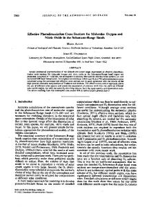
The problem of existence and uniqueness in problems involving collisions has a long and distinguished history, going back at least to Painlev´e [1895]. In these types of problems, the solutions are not continuous functions of time because of velocity jumps; they are also not continuous with respect to initial conditions. There is no general consensus about the best method for settling this issue; it is clear that the answer depends on how one precisely formulates it. We believe that our variational and algorithmic points of view can shed light on this question. Truesdell’s Example. We consider a problem suggested, and partially resolved, by Truesdell [1974]. The problem is that of a particle impacting the tip of a solid wedge with an acute angle, as shown in Figure 1.1. The particle is to reflect off the tip in a frictionless collision—the problem is to determine, in some rational way, what the particle will do when it hits the tip of the wedge. Two approaches that

Figure 1.1: Truesdell’s problem. have been quite unsuccessful in this area are, first, trying to make sense out of force/momentum balance and second, taking limits of smooth problems.

1

Variational Formulation. If one formulates the problem based on variational principles (which is consistent with the algorithmic formulation in Kane, Repetto, Ortiz and Marsden [1999]), then the solution is unique except for the singular initial condition where the velocity is pointing down the center of the axis of symmetry of the wedge, in which case there are two possible solutions. Thus, already in this simple example, one sees the advantage of a variational approach.

2

Nonsmooth contact algorithms

We shall be concerned with the motions of a deformable solid occupying a domain B0 ⊂ Rd in its reference configuration. The deformations of interest are described by deformation mappings ϕh : B0h ×[0, T ] → Rd subordinate to a finite element discretization of B0 . Here [0, T ] is the time duration of the motion. For a fixed t ∈ [0, T ], the deformation mappings ϕh (·, t) define a finite-dimensional space Xh . By a slight abuse of notation, we shall variously take ϕh to denote the discretized deformation field or the array of nodal coordinates in the deformed configuration. The Unconstrained Case. In the absence of contact constraints, the action functional for the solid is of the form   T 1 T ˙ h − φ(ϕh ) + f ext · ϕh dt ˙ h M hϕ I[ϕh ] = (2.1) ϕ 2 0 where M h is the mass matrix of the solid, φ(ϕh ) denotes its strain energy and f ext (t) are the externally applied forces. The equations of motion of the spatially discretized solid follow by requiring that I[ϕh ] ¨ h + f int (ϕh ) = f ext where f int = ∇φ(ϕh ) be stationary, with the resulting equation of motion M h ϕ ¨ h + f int (ϕh ) = f ext ) in conjunction with initial are the internal forces. The equation of motion ( M h ϕ ˙ h ]t=0 = ϕ ˙ h0 defines an initial value problem to be solved conditions of the form [ϕh ]t=0 = ϕh0 and [ϕ for ϕh . Time Discretization—Unconstrained Case. We envision an incremental solution procedure whereby ϕh is approximated at discrete times tn = n∆t. For definiteness, we specifically consider time-discretization algorithms belonging to Newmark’s family. See Belytschko [1983] and Hughes [1983]. Other timediscretization algorithms may be treated similarly. The time-discretized equations of motion are, therefore, of the form   ˙ n + ∆t2 (1/2 − β)ϕ ¨ n+1 ¨ n + βϕ ϕn+1 = ϕn + ∆t ϕ (2.2)   ˙ n+1 = ϕ ˙ n + ∆t (1 − γ)ϕ ¨ n + γϕ ¨ n+1 ϕ (2.3) ¨ n+1 + f int (ϕn+1 ) = f ext M hϕ n+1

(2.4)

˙ n+1 and ϕ ¨ n+1 . which defines a system of nonlinear equations to be solved for ϕn+1 , ϕ To complete the specification of our contact algorithm, we shall first develop some geometric and analytic tools. The Admissible Set. The notion of an admissible set of deformations will play a central role to extend the above procedure to nonsmooth contact problems. The admissible set Ch ⊂ Xh is simply the set of all globally invertible deformation mappings in Xh . Physically, ϕh ∈ Ch iff the deformation mapping ϕh does not entail interpenetration of matter: Ch = {ϕh : B0h × [0, T ] → Rd | gα (ϕh ) ≥ 0,

α = 1, . . . , N }

(2.5)

Kane et al. have also provided computationally efficient characterizations of the admissible set for spatially discretized solids by recourse to a collection of algebraic inequality constraints on the nodal displacements of the general form: gα (ϕh ) ≥ 0, α = 1, . . . , N , where N is the total number of possible contact constraints.

As is commonly done in so-called barrier methods, the interpenetration constraint may be accounted for by adding the indicator function ICh (ϕh ) of the admissible set Ch to the energy of the solid. The indicator of a set C is the extended-valued function IC (x) defined to be 0 for x ∈ C and ∞ otherwise. A complete account on nonsmooth analysis may be found in the monograph of Clarke [1983]. A brief review of concepts relevant to the present context has been given by Kane et al. [1998]. An approximate means of enforcing contact is by recourse to penalty methods. In the present context, a penalty formulation is N 1  obtained by approximating IC as: ICh (ϕh ) = [min{0, gα (ϕh )}]2 , where  is a small parameter. 2 α=1 The Constrained Case. Next we turn to the numerical treatment of nonsmooth contact problems. As is commonly done in so-called barrier methods, the interpenetration constraint may be accounted for by adding the term ICh (ϕh ) to the energy of the solid, whereupon the action functional becomes   T 1 T ˙ h M hϕ ˙ h − φ(ϕh ) − ICh (ϕh ) + f ext · ϕh dt (2.6) I(ϕh ) = ϕ 2 0 From the definition of the indicator function of a set it follows that the additional term in the energy effectively bars the trajectories from exiting the admissible set Ch , i. e., from violating the interpenetration constraint. The problem is now to determine the absolutely continuous trajectories ϕh (t) which render the action stationary (cf, Clarke [1983]). From the stationarity principle it follows that the trajectories are weak solutions of the equation ¨ h + f int (ϕh ) + ∂ICh (ϕh ) − f ext 0 ∈ M hϕ

(2.7)

˙ h ]t=0 = ϕ ˙ h0 ), defines an initial Eq. (2.7), in conjunction with initial conditions ([ϕh ]t=0 = ϕh0 , [ϕ value problem to be solved for ϕh . In eq. (2.7), the term ∂ICh (ϕh ) amounts to the contact forces over configuration ϕh . It follows from the invariance properties of Ch that ICh , and by extension the action I, is itself invariant under the action of translations and rotations. It therefore follows from Noether’s theorem (see, e. g., Marsden and Ratiu [1994]) that the solutions of (2.7) conserve linear and angular momentum. Global energy conservation follows likewise from the time independence or autonomous character  of the lagrangian. Additionally, since any admissible solution must necessarily be such that ICh ϕh (t) = 0, which corresponds to the fact that the contact area does not store or dissipate energy, it follows that the volume energy is also conserved. A Class of Nonsmooth Contact Algorithms. A class of time-stepping algorithms may now be obtained by treating (2.7) within the framework of the Newmark family of algorithms defined in (2.22.4). As in the case of plasticity (see, e. g., Ortiz [1981],[1983], and Pinsky [1983]), the robustness of the algorithm requires a fully implicit treatment of the contact force system ∂ICh (ϕh ). By contrast, the remainder of the terms in (2.7) may be treated either implicitly or explicitly. In view of this distinction, we ¨h = ϕ ¨ int ¨ con split the accelerations into terms due to the internal and contact forces, with the result ϕ h +ϕ h , where ¨ int ϕ h ¨ con ϕ h

ext = M −1 − f int (ϕh )] h [f

(2.8)

=

(2.9)

−M −1 h ∂ICh (ϕh )

A general class of implicit/explicit algorithms is obtained by setting: ϕn+1

2 ˙ n + ∆t2 [(1/2 − β)ϕ ¨ int ¨ int ¨ con = ϕn + ∆t ϕ n + βϕ n+1 ] + (∆t /2)ϕ n+1

(2.10)

˙ n+1 ϕ

˙ n + ∆t [(1 − = ϕ

(2.11)

¨ int γ)ϕ n

+

¨ int γϕ n+1 ]

+

¨ con ∆tϕ n+1

The explicit/implicit member of the algorithm, i. e., that which is explicit in the internal forces and implicit in the contact forces, corresponds to the choice β = 0. We shall refer to the remaining members

as being implicit/implicit. The above relations may be simplified by introducing the notation ¨ int ˙ n + (1/2 − β)∆t2 ϕ ϕpre n n+1 = ϕn + ∆t ϕ

(2.12)

2 int ¨ con ¨ n+1 + (∆t2 /2)ϕ ϕn+1 = ϕpre n+1 n+1 + β∆t ϕ

(2.13)

whereupon (2.10) becomes

Making use of the equation of motion (2.7), eq. (2.13) may be recast in the form 2 int 2 0 ∈ M h (ϕn+1 − ϕpre (ϕn+1 ) − f ext n+1 ] + (∆t /2)∂ICh (ϕn+1 ) n+1 ) + β∆t [f

(2.14)

which defines a system of nonlinear algebraic equations to be solved for ϕn+1 . Once this solution is ¨ int effected, the internal accelerations ϕ n+1 follow from (2.8) and the contact accelerations from (2.14), with the result ¨ con ϕ n+1 =

2 ¨ int (ϕ − ϕpre n+1 n+1 ) − 2β ϕ ∆t2 n+1

(2.15)

Finally, the velocities are computed from (2.11), which completes an application of the algorithm. Variational Structure. The crux of the algorithm just described consists of the determination of ϕn+1 from (2.14). The variational structure of this problem may be ascertained as follows. Begin by noting that (2.14) may be written in the form 0 ∈ ∂f (ϕn+1 ) + ∂ICh (ϕn+1 ) where, f (ϕn+1 ) =

1 pre ext (ϕ − ϕpre n+1 )M h (ϕn+1 − ϕn+1 ) + 2β[φ(ϕn+1 ) − f n+1 · ϕn+1 ] ∆t2 n+1

(2.16)

In the explicit case, β = 0, and f (ϕn+1 ) =

1 pre pre 2 (ϕ − ϕpre n+1 )M h (ϕn+1 − ϕn+1 ) = ϕn+1 − ϕn+1 K ∆t2 n+1

(2.17)

1 where v K = ∆t v T M h v may be interpreted as a kinetic-energy norm. The stable solutions of (0 ∈ ∂f (ϕn+1 ) + ∂ICh (ϕn+1 )) satisfy the minimization problem: min {f (ϕn+1 ) + ICh (ϕn+1 )} which ϕn+1 ∈Xh

is equivalent to the constraint minimization problem:

min

ϕn+1 ∈Ch

f (ϕn+1 ). This is a standard nonlinear

optimization problem, which may be solved by a variety of methods. One of the most successful methods, which we shall follow, for solving nonlinearly constrained optimization problems is the sequential quadratic programming (SQP) method. References for these methods are Spellucci [1993], Goldfarb [1983].

3

Extension to Frictional Contact

To account for frictional contact, we extend the force system in eq. (2.7) to include a frictional force field Rh , whereupon (2.7) becomes ¨ h + f int (ϕh ) + ∂ICh (ϕh ) − f ext + Rh 0 ∈ M hϕ

(3.1)

The frictional forces are required to be self-equilibrated and tangential to the surfaces in contact. We also assume that their magnitude depends on the normal pressure through Coulomb’s law of friction. The set Ch is characterized by the set of algebraic constraints gα (ϕh ) ≥ 0. Each constraint α corresponds to the intersection between a pair of distinct boundary simplices. The system of normal contact forces corresponding to constraint α may be written in the form: N α = λα ∇gα (ϕα ),

(3.2)

where λα is a scalar multiplier and ϕα are the local nodal position vector fields corresponding to each one of the contact constraints. Thus, ϕα is the collection of position vectors of the nodes attached to the pair of simplices involved in constraint α. The global system N h of contact forces is obtained by the assembly of all the local normal force systems {N α , α = 1, . . . , N } in the usual sense of finite elements. We denote this assembly operation symbolically as: N h = A({N α , α = 1, . . . , N }). Since the constraint functions are translation and rotation-invariant, it follows immediately that the local normal force systems are selfequilibrated, i. e., R(N α ) = 0; and M(N α ; ϕα ) = 0 The linear operators R and M are the resultant force and resultant moment of a system of forces. ˙ α be the local velocity field corresponding Next we introduce the concept of sliding velocity field. Let ϕ ˙ α is the collection of velocities of the nodes contained in the pair of simplices to the contact constraint α. ϕ ˙ α may include rigid-body components and may also include normal opening involved in constraint α. ϕ ˙ sli or closure modes. The corresponding local sliding velocity field ϕ α is found by extracting from the full ˙ α its rigid and normal components. Thus, ϕ ˙ sli local velocity field ϕ α is the solution of the local problem: ˙ sli ˙ α 2K minϕ˙ sli

ϕ α −ϕ α ˙ sli R(M α ϕ α ) = 0;

(3.3)

˙ sli M(M α ϕ α ; ϕα ) = 0;

˙ sli Nα · ϕ (3.4) α = 0.  where M α is the local stiffness matrix and we write v α K = v Tα M α v α . The first two constraints in (3.4) require that the sliding velocity field have zero total linear and angular momentum. The last ˙ sli constraint (N α · ϕ α = 0) is the orthogonality constraint. It ensures that the normal contact forces do no work on the sliding velocities. In view of (3.2), the orthogonality constraint may alternatively be ˙ sli expressed as ∇gα (ϕα ) · ϕ α = 0, which shows that the constraint function gα is left invariant by all ˙ sli ˙α sliding velocity fields, as required. From the linearity of the constraints (3.4) it follows that ϕ α and ϕ sli ˙ α = P α (ϕα )ϕ ˙ α It also follows that P α (ϕα )ϕ ˙ α is a projection which extracts are linearly related, i. e. ϕ the local sliding velocity field from the full local velocity fields. Clearly, the sliding velocity fields may be regarded as deformation modes, since they vanish identically under rigid-body motions. We introduce the local frictional force systems Rα by postulating the existence of a dual kinetic ˙ α ; ϕα ) or frictional dissipation function such that: Rα = ∂ψα∗ (ϕ ˙ α ; ϕα ) where the gradient potential ψα∗ (ϕ ˙ α , and the dependence of ψ ∗ on ϕα is regarded as parametric. In order that is taken with respect to ϕ ˙ α ; ϕα ) represent a true frictional dissipation function, i. e., that it be invariant under rigid-body ψα∗ (ϕ ˙ α ; ϕα ) is allowed to depend on ϕ ˙ α only through motions and sensitive to sliding only, the function ψα∗ (ϕ ˙ sli ϕ α For instance, in the case of Coulomb friction with coefficient of friction µ, we have: ˙ α ; ϕα ) = µ|N α (ϕα )||ϕ ˙ sli ψα∗ (ϕ α |

(3.5)

By construction of the sliding velocity fields, ψα∗ is invariant under rigid-body motions, so the local frictional force system Rα is self-equilibrated. In addition, from the orthogonality condition (∇gα (ϕα ) · ∗ ˙ ˙ sli ϕ α ; ϕα )) it follows that the local frictional forces Rα are orthogonal α = 0) and the relation (Rα = ∂ψα (ϕ to the local normal contact forces N α , as required. As in the case of the normal contact forces, the global frictional force system Rh appearing in the equation of motion (3.1) may now be constructed by assembling the local frictional fields, i. e. Rh = A({Rα , α = 1, . . . , N }). The global frictional force field inherits a potential structure from the local fields. Thus, we have ˙ h ; ϕh ) Rh = ∂ψ ∗ (ϕ

(3.6) N

˙ h ; ϕh ) = α=1 ψα∗ (ϕ ˙ α ; ϕα ) where the global frictional dissipation function is given by ψ ∗ (ϕ The resulting problem may be rendered in variational form as follows. Following Radovitzky and Ortiz [1999] and Ortiz and Stainier [1999], we begin by extending the effective energy (2.16) to account for friction by writing:

 ϕn+1 − ϕn pre 2 ext ∗ f (ϕn+1 ) = ϕn+1 − ϕn+1 K + 2β[φ(ϕn+1 ) − f n+1 · ϕn+1 ] + t ψ (3.7) ; ϕn+1 t The frictional variational problem is to find: minϕn+1 f (ϕn+1 ) with the following constraints: ϕn+1 ∈ Ch . We note that the variational principle just formulated is necessarily incremental, as required by the

dissipative character of the equations. Stationary of f (ϕn+1 ) with respect to ϕn+1 in the presence of constraint ϕn+1 ∈ Ch gives: 0∈

2 ext M h (ϕn+1 − ϕpre n+1 ) + 2β[f (ϕn+1 ) − f n+1 ] + ∂ICh (ϕn+1 ) + Rn+1 ∆t2

(3.8)

which may be regarded as a discretization of (3.1). The full displacement and velocity updates then follows from (2.10) and (2.11), with the accelerations computed from (2.8) and (2.15). A subtle point as concerns the algorithmic frictional force Rn+1 in (3.8) requires careful attention. Thus, in writing (3.8) we have identified the frictional forces with: 

 ϕn+1 − ϕn ∂ ∗ Rn+1 = t ψ ; ϕn+1 ∂ϕn+1 t



 ϕn+1 − ϕn ϕn+1 − ϕn = δ1 ψ ∗ (3.9) ; ϕn+1 + t δ2 ψ ∗ ; ϕn+1 t t A Comparison of this expression with (3.6) reveals that, in taking the full gradient of t ψ ∗ with respect to ϕn+1 we pick up the additional term t δ2 ψ ∗ not present in (3.6). For instance, in Coulomb’s model (3.5) this spurious term arises from the differentiation of the dependence of ψ ∗ on ϕn+1 introduced: by the projection of the local velocity fields onto their sliding components; and by the normal contact forces. However, it should be noted that the spurious second order term in (3.9) is of order O(t), and can therefore be regarded as an admissible contribution to the truncation error of the algorithm. In this manner Coulomb’s law of friction can be formulated in variational form as a minimum principle, despite its ‘non-associated’ character. Numerical tests and further analysis of this type of algorithm will be the subject of other publications.

References Belytschko, T. [1983] An overview of semidiscretization and time integration procedures Computational Methods for Transient Analysis, chap 1,1–65. Clarke, F. [1993] Optimization and Nonsmooth Analysis., Wiley and Sons, N.Y. Goldfarb, D. and A. Idnani [1983], A numerically stable dual method for solving strictly quadratic programs, Mathematical Programming,27, 1–33. Hughes, T.J.R. [1983], Analysis of transient algorithms with particular reference to stability behavior, Computational Methods for Transient Analysis, 67–155. Kane, C., E.A. Repetto, M. Ortiz and J.E. Marsden [1999] Finite element analysis of nonsmooth contact Computer Meth. in Appl. Mech. and Eng., 180, 1–26. Marsden, J.E. and T.S. Ratiu [1994] Mechanics and Symmetry. Texts in Applied Mathematics, 17, SpringerVerlag, Second Edition, 1999. Ortiz, M. [1981], Topics in constitutive theory for inelastic solids, PhD thesis - University of California at Berkeley . Ortiz, M., P.M. Pinsky and R.L. Taylor [1983] Operator split methods for the numerical solution of the elastoplastic dynamic problem, Computer Methods in Applied Mechanics and Engineering, 39, 137–157. Ortiz, M. and L. Stainier [1999]. The variational formulation of viscoplastic constitutive updates. Computer Methods in Appl. Mech. and Eng., 171, 419–444. Painlev´e, P. [1895] Sur les lois du frottement de glissement. C.R. Acad. Sci., Paris, 121, 112–115, 140 (1905), 702–707, 141 (1905), 401–405 and 546–552. Pinsky, P.M., M.Ortiz and R.L. Taylor [1983], Operator split methods for the numerical solution of the finitedeformation elastoplastic dynamic problem, Computers & Structures, bf 17, 345–359. Radovitsky, R. and M. Ortiz [1999]. Error estimation and adaptive meshing in strongly nonlinear dynamic problems. Computer Methods in Appl. Mech. and Eng., 172, 203–240.

Spellucci, P. [1993], A new technique for inconsistent QP problems in the SQP method, Technical University at Darmstadt. Truesdell, C. [1974] A simple example of an initial-value problem with any desired number of solutions. Ist. Lombardo Accad. Sci. Lett. Rend. A 108, 301–304.