Tactile Object Recognition From Appearance Information

1

Tactile Object Recognition From Appearance Information Zachary Pezzementi, Student Member, IEEE, Erion Plaku, Caitlin Reyda, Gregory D. Hager, Fellow, IEEE

Abstract—This paper explores the connection between sensorbased perception and exploration in the context of haptic object identification. The proposed approach combines (i) object recognition from tactile appearance with (ii) purposeful haptic exploration of unknown objects to extract appearance information. The recognition component brings to bear computer vision techniques by viewing tactile sensor readings as images. We present a bag-of-features framework that uses several tactile image descriptors, some adapted from the vision domain, others novel, to estimate a probability distribution over object identity as an unknown object is explored. Haptic exploration is treated as a search problem in a continuous space to take advantage of sampling-based motion planning to explore the unknown object and construct its tactile appearance. Simulation experiments of a robot arm equipped with a haptic sensor at the end-effector provide promising validation, indicating high accuracy in identifying complex shapes from tactile information gathered during exploration. The proposed approach is also validated by using readings from actual tactile sensors to recognize real objects.

I. I NTRODUCTION Tactile force sensors, consisting of an array of individual pressure sensors, are becoming common parts of modern manipulation systems. It is generally expected that a new robotic hand design will include tactile force sensors embedded in each fingertip and possibly along other surfaces of the hand. The current generation of tactile sensors is also much more capable than previous generations. Resistive sensors are commercially available at resolutions as high as 40x40 per square inch [1], capacitive sensors offer greatly-increased force resolution and repeatability, and recent optical gel sensors [2] offer remarkably high resolutions that depend primarily on the camera being used, size, and other methodological trade-offs between spatial and depth resolution. Given the advancement and ubiquity of tactile force sensors, it becomes important to be able to extract as much information as possible from these sensors about the task at hand. In this work, we use the object recognition task as a benchmark for evaluating the quality of various ways of interpreting tactile force sensor readings. We develop a method to distinguish between objects using only the responses of tactile sensors and compare several representations of tactile information for Zachary Pezzementi and Gregory D. Hager are with the Department of Computer Science and the Laboratory for Computational Sensing and Robotics, Johns Hopkins University, Baltimore, MD 21218. Email: {zap, [email protected]}. Erion Plaku is with the Department of Electrical Engineering and Computer Science, Catholic University of America, Washington, DC 20064. Email: [email protected]. Caitlin Reyda is with the Department of Mechanical Engineering, Massachussetts Institute of Technology, Cambridge, MA 02139. Email: [email protected].

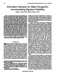
(a) Tactile exploration in simulation

(b) Tactile images

Fig. 1. Depiction of a chess piece being explored by our simulated robotic arm (shown in dark blue) and tactile sensor system (shown in purple). Note that the tactile exploration method does not know the position, orientation, or the geometry of the object. Yellow patches show the sensor placements at which local controllers converged and a local appearance feature was extracted and recorded. The corresponding tactile images are shown to the right.

this purpose. The effectiveness of the method is demonstrated by recognizing a set of complex 3D objects in simulation and a set of raised letters both in simulation and using real sensors. Our general approach is to interpret tactile sensor readings as “tactile images”, which measure a patch of the surface of an object. In previous work, we characterized a set of tactile sensors from Pressure Profile Systems [3] and developed a simulator to emulate that class of tactile sensors’ response in interactions with rigid objects [4]. Tactile sensors were found to be modeled well as camera systems that detected depth information, modified by a point spread function dependent on the thickness of a covering material. Now we use the same sensor model, but expand the simulation to include the full robotic exploration task, with tactile sensing as the sole form of feedback, as illustrated in Fig. 1. By thinking of sensor readings as images, we bring to bear a large body of work from computer vision. The interpretation of the information in these force images is somewhat simpler than in the visual case, since there are no perspective effects and there is only one channel of intensity information. The collection of images, however, is considerably more difficult, since each small patch must be obtained by actively interacting with the environment, while hundreds of features can be extracted from a single passive image in the visual case. In order to get useful tactile force readings, we draw from recent advances in sampling-based motion planning [5]–

2

[13] to design effective exploration strategies of the surface of an unknown object that ensure good local and global coverage. The exploration leverages the idea of selectively sampling the robot workspace to guide the exploration towards unexplored parts of the workspace and locally explore areas where it collects measurements. Since the exploration does not rely on knowing the position, orientation, and geometry of the object, it is suitable even when the unknown object is perturbed between sensor readings, e.g., as a result of robot manipulations. The only requirement is that the object remain relatively stable while taking a sensor measurement. Once the sensors are near the surface, they are pressed down under closed-loop control to maximize the information content of the resulting images. Due to these differences in the image formation process, it is not obvious how much of our knowledge of visual images will be transferable to tactile images. Accordingly, we take the approach of adapting and testing a variety of promising methods from the vision literature, as well as developing novel ways of representing tactile information. We are interested specifically in the interpretation of tactile images, which describe local surface appearance. We have therefore isolated the appearance portion of the object recognition task from its geometric counterpart to better observe the effects of changes in the appearance representation. Inspired by the success of bag-of-features techniques in the vision domain, we present an appearance-based recognition algorithm adapted to the domain of tactile data. Appearanceonly algorithms are particularly useful for systems which cannot accurately measure the positions at which contacts are made, or if the object is perturbed during exploration. A good understanding of information provided by appearance alone will also better inform the design of algorithms that also use geometry information, minimizing the data needed to identify objects which cannot be discriminated with appearance or geometry information alone. The bag-of-features algorithm is applied to the images collected during exploration to maintain an online estimate of the probability of object identity, as illustrated in Fig. 2. The system is, therefore, able to output its best guess at object identity, as well as its confidence in that identification (as a full confusion matrix, if desired), at any given time in the exploration. Experiments demonstrate the discriminative power provided by only a small number of sensor readings with this framework. Performance continues to increase with more readings, as a better estimate of the appearance distribution can be modeled. II. R ELATED W ORK Although object recognition has been widely explored in the vision literature, haptic approaches have received relatively little attention, probably due to the inadequacy of available sensors. Early approaches focused almost entirely on producing clouds of contact points to constrain the geometry of the object [14]–[18]. Several researchers made use of tactile sensors, but typically only for the purpose of localizing contact points or estimating surface normals associated with each

contact point [18]–[22]. Whereas these methods rely almost entirely on the location and net force produced by contacts, in order to reduce the impact of perturbations, our work takes a different approach and relies instead on tactile appearance. Other work has focused on extracting simple shape features such as lines, points, or corners [23]–[25], but application of such features to recognition has been largely heuristic, requiring hand tuning for each object. Some researchers have instead employed hybrid techniques, supplementing haptic sensing with information from vision systems [26]–[29]. At the same time, some of the most successful object recognition systems in the vision literature are based on local features, often without any associated geometry information [30]–[32]. A recent overview of this work is provided in [33]. These “bag-of-features” methods typically sample small patches of an image and use one of several descriptors to extract feature vectors from these patches, then represent objects as producing distributions over these feature vectors. Although the performance of local descriptors has been comprehensively studied on visual data [34], [35], no work we are aware of has yet applied these techniques to tactile data. Interestingly, a recent psychophysical study indicates humans may also use local feature-based processing for tactile recognition [36]. We develop novel methods for adapting the feature-based approach to haptics and demonstrate its effectiveness in the new domain. The recent work by Schneider et al. [37] is most closely related to ours, since it also applies bag-of-features to data from tactile force sensors. The work presented in this paper goes farther than Schneider et al. in several important ways. In their experiments, the pose of the objects is always known, considerably simplifying both the recognition problem and the process by which sensor readings are collected. The latter is treated as simply the selection of the height at which to grip the object. In this work, however, we leave the object pose as unknown (bounded only to be within the robot workspace) and we present exploration algorithms to collect consistent sensor readings in the face of this additional challenge. Additionally, Schneider et al. simply use the raw tactile sensor images as features, whereas we investigate several possible descriptors for extracting informative features. Some of the work above has addressed the issue of how to conduct haptic exploration of an unknown object, but generally with the goal of constraining the object’s geometry, rather than that of collecting informative and consistent tactile force readings. Schneider et al. discuss the selection of maximallyinformative grasps using entropy minimization, but they do not address the gripping process or its effect on the resulting tactile images. In the appendix of [38], Kraft et al. describe a pair of PI controllers for collecting tactile force sensor readings with consistent applied force and orientation, with the goal of estimating the surface normal. We derive a new but similar set of controllers that also align the tactile sensor with the object surface normal and apply a target force with the goal of extracting consistent sensor readings of a given patch of object surface.

3

Global Search Target Local Search

Surface Contact Reading Controllers

Appearance Modeling

Identity Estimate

Fig. 2. Illustration of exploration process for collecting each sensor reading.

III. E XPLORATION When exploring an unknown object, the objective is to collect sensor measurements from various locations on the object surface that would enable the recognition method to identify the unknown object. The fact that there is no a priori information about the position, orientation, and the geometry of the unknown object makes the exploration more challenging. Only the workspace boundaries of the robot are known, and it is assumed the object is somewhere within these bounds. The exploration is carried out in a simulator, which models the robot (as an articulated arm) and the behavior of the haptic sensor, which is attached to the end-effector. Details of the simulator can be found in section V-A. Exploration strategies employed in this paper vary from local strategies that attempt to cover one area and then move on to explore the next neighboring area, to global strategies that attempt to take sensor measurements from all over the surface of the unknown object. Exploration makes use of a local controller, which enables the robotic system to take consistent sensor measurements regardless of the sensor’s angle of approach to the surface of the unknown object. The rest of this section describes in more detail the exploration strategies (section III-A) and the local control (section III-B). A. Strategies to Explore the Unknown Object Drawing from sampling-based motion planning [5], [6], the underlying idea in exploration is to sample various poses inside the robot workspace and compute collision-free motions that move the robot arm so that the sensor achieves the desired pose. The planner maintains a tree data structure, which is rooted at the initial configuration of the robot arm. The tree vertices consist of collision-free configurations, while edges indicate collision-free motions between the configurations that they connect. The planner employs two strategies to grow the tree, one geared towards global exploration and another towards local exploration. At each iteration, the planner makes a probabilistic selection of which strategy to use; the local strategy is selected with probability L and the global strategy is selected with probability 1 − L. A study of the impact of L on the overall performance is presented in section V. To guide the exploration to obtain a global view, the planner samples a target position p uniformly at random inside the workspace boundaries. Then the planner selects the configuration q from the tree whose associated sensor location is closest to p. This strategy, drawing from the rapidly-exploring random tree [7] algorithm, has the effect of pulling the exploration toward new and different locations to ensure global coverage. To guide the exploration based on local coverage, the planner imposes an implicit uniform grid over the workspace.

Each time the sensor makes contact with the unknown object and a measurement is taken, the location ` of the sensor is added to the corresponding grid cell. In this way, each grid cell maintains a list of locations from which sensor measurements have been taken. From the list of non-empty grid cells, a cell c is then selected with probability inversely proportional to the number of measurements taken from locations inside that cell. Thus, the planner gives preference to cells that have few measurements, since further exploration of these cells may increase the local coverage. The planner then selects a location ` uniformly at random from all the locations associated with c and samples a target position p uniformly at random inside a small sphere centered at `. The configuration from which to expand the tree is then selected as the configuration in the tree that is closest to p. In this way, the planner attempts to increase the local coverage of the selected cell and move the exploration toward neighboring areas. After a configuration q in the tree and a target position p are selected, the objective of the planner is to expand the tree from q toward p. Recall that the planner only knows the workspace boundaries and has no a priori information about the position, orientation, and the geometry of the unknown object. For this reason, the planner takes small steps toward p. In particular, at each iteration, the planner computes the direction from the location of the sensor to p and attempts to move in that direction to a nearby point p0 . The planner employs numerical inverse kinematics to compute the configuration q 0 that places the sensor at location p0 . The planner then relies on a controller to slowly move the robot arm from configuration q to q 0 . If at any time during this movement the object is sensed, the planner switches to the surface contact control scheme, which is described in the next section, to obtain a measurement. As evidenced by the experiments, this combination of local and global strategies allows for an effective exploration of the surface of the unknown object. The exploration process is illustrated on a 3D model of a chess piece in Fig. 1, which shows where 100 tactile images were extracted using the planner, alongside depictions of the first 50 of these images. We also note that, since the exploration strategy does not rely on knowing the position, orientation, and geometry of the object, the exploration strategy is suitable even when the unknown object is perturbed between sensor readings, e.g., as a result of robot manipulations. In fact, such motions have no effect on the global strategy, since the global strategy is guided by uniform sampling inside the workspace. The effect on the local strategy is also minimal. If the planner takes a sensor measurement at location `, it will attempt to take another sensor measurement at a target position p sampled uniformly at random inside a sphere centered at `. As such, even if the unknown object is perturbed when taking a sensor measurement at `, it is likely that it moved locally so that sampling in a local neighborhood of ` is generally suitable to accommodate such motions. As the experiments indicate in Section V-B4, the overall approach remains effective even when the unknown object is perturbed between sensor readings.

4

Start

Estimate Surface Normal

Start

No

Approach

Error < T?

No Done?

Yes

Done?

(b) Orient

Orient

Done

Yes

(a) Overall

No Error < T?

Start

Done?

End

Saturated?

Move Forward

Yes

No

Orient

Yes

No

No

Yes

Not Done

Done

No Done?

Start

Yes

Yes

Press

Rotate Towards Estimated Normal

Approach implements essentially a guarded move, terminating as soon as any sensor element response goes significantly above zero. Press is implemented as a PD controller with a second termination criterion if any single sensor element becomes close to fully saturated. The Orient controller operates by fitting a plane to the pressure readings of the individual sensor elements (implicitly fitting a plane to the surface being sensed) and commanding the robot to re-orient the sensor normal to the plane fit normal, as shown in Algo. 1. This process is repeated until either the normals converge to within a thresholded angle of each other or a maximum number of iterations is reached.

No Contact?

Move Forward

Not Done

(d) Press

Yes Done

Not Done

(c) Approach Fig. 3. Surface contact controller flow charts. (a) shows the flow of control between local controllers, and (b), (c), and (d) depict the individual controllers.

B. Surface Contact Control The objective of the surface contact control scheme is to extract a consistent descriptor each time a sensor measurement is taken at a given object location, regardless of the sensor’s angle of approach to the surface, to provide the object recognition scheme with reliable estimates of the local surface properties. Because of the small field of view of typical tactile sensors, normalization of the image with respect to the contact pose cannot be expected to be achievable solely through post-processing of the resulting images. Therefore, to achieve measurement consistency, some level of closed-loop control is necessary. The entire control scheme used in this portion of the exploration process is illustrated in Fig. 3a. Three local controllers are used to establish consistent sensor poses. All controllers use the output of the tactile sensor to compute commands for the robot arm. The overall strategy begins with the Approach controller (Fig. 3c), which moves the sensor in a given direction until it comes into contact with the object. Achieving contact then engages the Press controller (Fig. 3d), which continues to move the sensor along the same axis until the average pressure of all sensor elements. Then the Orient controller is engaged to bring the sensor as close to coplanar with the object surface as possible. Finally, control is passed sequentially back and forth between Press and Orient until both controllers consecutively issue no command. While it would be possible to implement surface contact control using standard closed-loop force feedback controllers, with the variety of goals and the complexity of making and breaking contact, we found a step-wise formulation to be useful. The Approach and Press controllers’ implementations are fairly straightforward, while that of Orient is more involved.

Algorithm 1 Orient Controller 1: 2: 3: 4: 5: 6: 7: 8: 9: 10: 11: 12: 13: 14:

pts ← ∅ for all sensor elements i do if val(i) > contactT hresh then p ← point3D(getX(i), getY (i), estimateDepth(val(i)) add p to pts end if end for normal ← f itP lane(pts) sensorN ← toW orldCoords(point3D(0, 0, 1)) surf aceN ← toW orldCoords(normal) step ← 0.3 target ← step · surf aceN + (1 − step) · sensorN cmd ← rotationF romT o(sensorN, target) return cmd

It can be seen later in the experiments (Figs. 5 and 6) that these controllers converge upon features such as edges and corners as well as flat surfaces. Their convergence characteristics are analyzed quantitatively in the presence of noise in section V-C. IV. I NTERPRETING TACTILE DATA Each tactile image obtained during testing or training is converted into a feature vector for further processing. Drawing from the computer vision literature, we make use of image descriptors that have worked well for a wide variety of recognition problems, as described in section IV-B. The objective of the image descriptors is to extract the most relevant information for characterizing the local surface properties. Moreover, since surface contact controllers (section III-B) control for orientation except about the axis normal to the sensor surface (and this angle is not recorded), the descriptors need to be invariant to rotations about this axis. The extracted features are then used in the recognition process, as described next. A. Bag-of-Features Modeling A bag-of-features approach [33] is developed to model the appearance of objects. The major steps of the process for learning this model (Training) and for applying it to recognition (Testing) are illustrated in Fig. 4. Let O1 , . . . , OnO denote the object classes used for training. For each object class Oj , a set {Ij,1 , . . . , Ij,nI } of nI images are collected via the exploration procedure described in section III. Then for each descriptor d, a set of features Fj = {fj,1 , ..., fj,nF j } is extracted for all of the images from

5

Training

This minimization can also be interpreted as a maximization of the likelihood of the data over object identity, as shown in the Appendix. Other methods of comparing histogram distributions, such as histogram intersection and χ2 , were also considered, but experiments indicated that the above formulation gave significantly better results. This formulation is also more easily adaptable to integration with a guided search framework for evaluating the potential information content of future measurements and choosing an appropriate exploration strategy.

Testing

Collect Images of Each Class

Collect Images of Unknown Object

Extract Descriptors

Extract Descriptors PCA Transform

PCA

Cluster

Compute Cluster Memberships

Cluster Model

Build Per-Class Histograms

Apply PCA Transform

Class Histograms

B. Descriptors

Histogram Comparison

Class Probability Estimates

Fig. 4. Process for learning bag-of-features models for each object class and applying them to classify unknown objects.

object class j, with the features from each image denoted d(I). The features are then reduced in dimensionality by using PCA and discarding the least significant components that account for up to 10% of the variance. The reduced feature vectors are then grouped into clusters {c1 , . . . , cnC } by a learned clustering function, C(f ), which takes a feature, f , and outputs its cluster membership. The choice of an appropriate clustering method is discussed further in section V-B1. During testing, the data consist of images obtained by the exploration procedure in section III-A. Descriptors are extracted from each image, as in training, then their dimensionality is reduced with the PCA transform from training. Finally, the cluster membership function obtained in training is applied to the descriptors to form an empirical distribution on cluster membership. This process gives a histogram representing the probability of drawing observed features U = {u1 , ..., unU } from each cluster given data from the unknown object, which is denoted as p(ci |U). Then, given an estimate of p(ci |Oj ) from training, the bestmatching object identity, D, is taken as that which minimizes the K-L divergence [39] between the distributions p(ci |Oj ) and p(ci |U), D = min DKL (p(ci |U) ||p(ci |Oj ))

(1)

p(ci |U) p(ci |Oj )

(2)

p(ci |U) log p(ci |Oj )

(3)

j

DKL (p(ci |U) ||p(ci |Oj )) =

X

p(ci |U) log

i

=

X

p(ci |U) log p(ci |U) −

i

X i

Since p(ci |U) is fixed in the optimization, the first term can be dropped, leaving X D = argminj − p(ci |U) log p(ci |Oj ) (4) i

Several different descriptors, as described below, are considered for representing the essential information from the sensor readings in an intensity- and rotation-invariant way. We first present the descriptors that are adapted directly from their counterparts in the computer vision literature, SIFT and MR8. The remaining descriptors are novel. We also investigated additional vision-inspired descriptors based on steerable filters [40] and the Schmid texture descriptor [41], but they have been omitted due to poor performance. 1) Vectorize: Takes a tactile image and concatenates its columns to form a vector. The result should not be rotationinvariant unless the images happen to be rotationally symmetric. This is our negative control, and can be considered a “do-nothing” descriptor, inspired in part by [42], to show a baseline performance level provided by the rest of the method. 2) SIFT: SIFT features have been shown to perform extremely well in visual texture discrimination [34], [35]. We follow many others in the vision community (e.g. [43]–[45]) by applying only the descriptor portion of the SIFT algorithm to characterize image patches. This practice seems particularly appropriate since the tactile images already represent patches of the object surface. The standard SIFT descriptor [46] is used, as implemented in the VLFeat library [47], at a scale corresponding to the size of the image and orientation derived in the standard SIFT way. To avoid histogram sparsity issues, the computation was switched from a 4x4 to a 2x2 grid of sampling areas at low resolutions, giving a 32-element vector rather than the usual 128. However, no significant differences in performance were observed in this context, as compared to using the full 128-element descriptor, even for the smallest images. 3) MR-8: Varma and Zisserman compared various filter sets for texture classification, and we chose their best-performing filter set, MR-8 [48], as one of our descriptors, as implemented by [49]. The Maximal Response set consists of first- and second-order derivatives of oriented Gaussians at different scales and angles as well as a symmetrical Gaussian and difference of Gaussians. Rotational invariance is achieved by only taking, from the set of all angles for each oriented filter, that with the largest-magnitude response, on a pixel-by-pixel basis. The oriented filters consist of 3 scales and 2 orders of derivatives, evaluated at 6 angles each. So taking the maxima of these gives 6 responses, plus the two symmetric filters’ responses, for a total of 8. The responses of subsections of the tactile image to all 8 of the filters selected by the process

6

above are concatenated to form feature vectors. Then the set of feature vectors from all sections of the image (4 overlapping sections in the 6x6 case) are returned as the image’s descriptor. This descriptor is unique among those presented in this work in that it returns multiple feature vectors for each input tactile image. It is also, however, by far the most computationally expensive, particularly for large images. 4) Moment-Normalized: First, the image is masked so that only pixels within the largest inscribed circle about the image center are retained. Then, following Hu [50], the descriptor computes spatial moments for the image with respect to the image center (not its center of inertia), normalizes them for scale, and extracts the image’s principal axes. The angle of the major axis is taken as a measure of orientation, and the 180 degree ambiguity is resolved with the use of the sign of a 3rd-order moment (again from [50], though this may still fail for certain types of symmetry). The image is then rotated spatially with bilinear interpolation so that the computed major axis direction is aligned with the positive-X-axis. Finally, the resulting image is converted to a vector as in Vectorize. It should be invariant to intensity changes and rotation, though local control should have already eliminated most intensity variations. 5) Polar-Fourier: The descriptor begins by masking out the corners of the image, as in the moment-normalized descriptor. Then the image I is re-sampled using polar coordinates to produce a new rectangular image IP whose axes are radius and angle. Let (x0 , y0 ) be the center of the original image, D be the diameter of the image’s largest inscribed circle, and i i , θ = 2πj and j vary as {1, 2, . . . , D}. Then r = 2D D , and IP (i, j) = I (x0 + rcos(θ), y0 + rsin(θ)) ,

(5)

where I(x, y) indexes the original image’s pixels. In this way, each row of this image corresponds to a single radial distance, and moving across columns traces out a circle. Between each consecutive pair of rows of this image, two new rows are added, corresponding to the sum and the difference of the surrounding rows, to form IQ : IQ (3i, j) = IP (i, j) (6) IP (i, j) + IP (i, j) IQ (3i + 1, j) = (7) 2 IP (i, j) − IP (i, j) IQ (3i + 2, j) = (8) 2 The Fourier transform of each row of this new image is taken, and the magnitudes of the resulting coefficients are recorded. Since, in the Fourier domain, a rotation about the image center results in only a change in phase, discarding that phase information leaves only the coefficient magnitudes, which should be invariant to rotation. Rotations only cause a particular family of phase changes, though, so discarding phase information completely also allows many other transformations, such as independent rotations of the various “rings” of the original image represented by the rows of the polar representation. The extra rows added to form IQ serve to provide information on how adjacent rings of the original image were related, to mitigate the effects of losing such relationships when discarding the phases of the Fourier components in this polar

space. From these coefficients, a vector is formed by choosing the N lowest-frequency coefficients from each row, where N is proportional to the radius at which that row’s points were sampled, rounded to the nearest whole number. This sampling of coefficients is intended to correspond as closely as possible to a uniform sampling of the original image, which became over-sampled toward the center of the image in the conversion to polar coordinates. 6) MNTI: Finally, we also include a modification of the Moment-Normalized descriptor to be invariant to translations, which is referred to as moment-normalized translationinvariant (MNTI). This descriptor follows the same procedure as Moment-Normalized up to the final vectorization step. Then, MNTI is obtained by taking a 2D spatial Fourier transform, recording only the magnitudes of each Fourier component and vectorizing the result. As in the previous descriptor, discarding the Fourier phase has the effect of adding invariance to a set of transformations. Since we are taking the 2D transform in the original image space, this includes the set of 2D translations (once more along with many others). Application of the Fourier transform, however, assumes the image is a repeating signal that wraps around at the image boundary. Therefore, in order to mitigate ringing effects at the boundary, the moment-normalized image is first padded to 150% its original size, and these new pixels are set to values linearly interpolating between the original image’s boundary pixels and zero. V. E XPERIMENTS AND R ESULTS The experiments highlight the effectiveness of the proposed framework in recognizing unknown objects from sensor measurements gathered during exploration. The experiments indicate a high degree of recognition accuracy for various simulated shapes. In addition to strong performance in simulation, the proposed framework is shown to be effective in recognizing objects based on real sensor measurements. A. Experimental Setup 1) Simulated Robotic System: The simulated robotic system consists of an articulated arm equipped with a haptic sensor at the end-effector. In its initial configuration, the first link of the robotic arm is perpendicular to the xy-plane and all the other links are perpendicular to the yz-plane. Any two consecutive links of the robotic arm are connected by a joint that allows rotations about the y- and z-axes. The haptic sensor is connected to the last link via a universal joint. This particular robotic system was chosen to provide a concrete setup for developing and testing the exploration strategies. Note, however, that the exploration strategies in this paper are general and can be used with any robotic system for which forward kinematics are available. 2) Simulated Haptic Sensor: The tactile sensor is simulated by the method described in our previous work [4]. In brief, the sensor is modeled as an orthographic camera whose viewing volume is defined by a layer of deformable material covering the sensor. Simulated 3D objects are allowed to penetrate this covering, and the penetration depths are measured by the

7

simulated camera to generate a depth image. A point spread function is then applied to this image, with parameters dependent upon the physical properties of the covering material. The resulting image is then discretized to the resolution of the tactile sensor being simulated to generate the final tactile image. More details can be found in the original paper [4]. 3) Data Collection During Training: Note that the planner (section III) is employed only during the testing stage of the framework when the objective is to identify an unknown object from various sensor measurements taken during exploration. During the training stage, the position, orientation, and geometry of the object are known, so much simpler strategies can be used to collect measurements. In particular, measurements during training are collected by placing the sensor at various locations close to the surface of the object and then allowing the local controllers to converge. More specifically, first a triangle is selected from the triangular mesh with probability proportional to its area. A point p is then sampled uniformly at random inside the selected triangle and the point p is then moved back some distance in the direction opposite the triangle normal. The sensor is then placed at this location facing toward the triangle. A small perturbation is applied to the sensor orientation and then the local controllers are used to approach the surface and take a measurement. This process is repeated until a specified number of sensor measurements are obtained. In this way, the exploration strategy during training is computationally fast and allows us to obtain extensive coverage of the object.

membership function that can be applied to new data after training, which removed many algorithms from consideration. We began by applying k-means repeatedly with various values of k, to mitigate sensitivity to initialization conditions. Performance during this process was measured using a validation set, consisting of data reserved from the training set. The “best” model was maintained as that which displayed the highest classification accuracy on the validation set. Since classification accuracy was a relatively coarse measurement, ties were broken by considering classification reliability, the total probability weight allocated to correct classes. In order to visualize the clustering results, the cluster centers were back-projected through PCA and then reshaped into the original image space. This is only possible with the Vectorize and Moment-Normalized descriptors, as the others involve a loss of spatial information that prevents reconstruction of a unique representative image. Inspecting the cluster centers resulting from k-means revealed several clusters which either seemed redundant or appeared not to correspond to real data points. These effects motivated investigation of soft clustering techniques to mitigate the discretization inherent in k-means, so we then turned to Gaussian mixture models (GMMs). We began with the same image descriptors as in k-means, reduced in dimensionality with PCA. A single mixture model with k components was fit to the data. Let a GMM, G, consisting of nG components, {g1 , g2 , . . . , gnG }, be defined as nG X P (x|gi )p(gi ) (9) P (x|G) = i=1

B. Simulation Experiments with 3D Objects The effectiveness of the framework was first tested on various simulated shapes. The effect of different clustering methods as well as the choice of descriptor under several resolution, noise, and covering configurations were also evaluated. These simulation experiments allowed us to select good parameters for the framework before applying it to real objects and sensors. For the simulation experiments, a set of 10 shapes from the Princeton Shape benchmark was used, as shown in Fig. 5. The sample shapes were selected to traverse several domains and to present a variety of interesting surface geometries, in order to cover a large portion of the range of local appearance characteristics that descriptors would need to represent. For training, the sampler (section V-A3) was used to collect 1000 tactile images of each object for learning models of the objects, plus another 100 samples of each object to form a validation set that was used to evaluate performance during the training process. Then for testing, the planner (section III) was used to collect a further 100 samples of each object which were compared with the learned models. This testing stage was then repeated 3 times, and the results were averaged to smooth out inconsistencies due to small amounts of data. 1) Clustering: A variety of clustering methods were evaluated for forming the bag-of-features models. The standard k-means approach was used as a starting point, with the initialization method described in [52]. We considered it essential that the clustering algorithm provide an efficient

P (x|gi ) = N (µi , Σi ),

(10)

where N (µi , Σi ) represents a multi-dimensional normal distribution parameterized by mean µi and standard deviation Σi . In order to compute the cluster membership defined in section IV-A, this set of probabilities was interpreted as a soft binning function into a histogram where each bin corresponds to a mixture component. The likelihood of each cluster, ci , associated with the object’s entire feature set, F = {f` }, is computed as X p(ci |F) = λ p(f` |gi )p(gi ) (11) `

where λ is a normalization constant. Sets of data points were then “binned” and summed to form histograms of cluster/component representation, which were compared using the same method described in section IV-A. A sampling of 48 cluster centers using the Moment-Normalized descriptor is shown in Fig. 6. As in the k-means case, the mixture component means are back-projected through the PCA transformation and reshaped into the original image space. The differing covariances associated with each mixture component add additional information to this clustering result, but they are not visualized here. The phenomenon mentioned above can still be observed to some extent, but soft membership allows weighted association with all clusters simultaneously, imparting much more information than discrete association with a single (potentially outlier) cluster. Accordingly, performance using GMMs was substantially higher, but so was computation time.

8

(a) Skull

(b) Glass

(c) Tire

(d) Chair

(e) Pliers

(f) Screwdriver

(g) Knight

(h) Dragon

(i) Helmet

(j) Phone

Fig. 5. The set of models from the Princeton Shape Benchmark [51] used for testing. Some are shown as wire-frames or colored for clarity, but only geometry information was used in experiments. Below each is a sampling of 30 6x6 tactile images measured from that object during training.

Fig. 6. A sampling of cluster centers from training on the Princeton set with the Moment-Normalized descriptor. Each image represents the mean of a Gaussian mixture component, back-projected into the original 6x6 tactile image space.

2) Descriptor Comparison: Fig. 7 compares the performance of the various descriptors on the set of Princeton models, as a function of the number of tactile readings of the object surface that were sampled. In this format, which is used for all our graphs, each data point tells the empirical probability of correctly identifying any unknown object given that number of samples of its surface, using the indicated descriptor. More samples tend to give a better estimate of the true appearance distribution, leading to higher recognition accuracy, but adding non-representative samples can also lower accuracy. The descriptors taken directly from the vision literature (SIFT and MR) gave poor results, generally no better than simply using the original image (Vectorize). Polar-Fourier and MNTI perform best in terms of classification accuracy, followed by the Moment-Normalized descriptor. For this reason,

Fig. 7. Comparison of various descriptors on Princeton set at 6x6 resolution and 10% covering thickness.

only the performance of these top 3 descriptors (PF, MNTI, and MN) and Vectorize are shown for subsequent tests, though this performance trend was verified to continue under other sensor configurations. Polar-Fourier and MNTI performed consistently and about equally well in nearly all our tests, despite having rather different formulations. Both, however, make use of the magnitudes of Fourier coefficients to obtain invariance with respect to a class of image transformations (and therefore the corresponding physical transformations). Despite the fact that there is a significant loss of information in this process, the invariance

9

(a) MNTI

(b) Polar-Fourier

Fig. 8. Comparison of different exploration strategies by varying L on Princeton set at 6x6 resolution and 10% covering thickness.

(a) Moment-Normalized

(b) Polar-Fourier

Fig. 9. Performance of MN and PF on validation data for the tests of section V-B6. The validation data were collected using the sampler of section V-A3, whereas test data were collected using the full planning algorithm of section III. Performance on the validation data is much stronger.

gained seems to consistently increase performance. 3) Exploration Strategy: We also examined the trade-off between global and local exploration by varying a parameter L, to select between the two exploration strategies described in section III-A. L defines the probability at each iteration of exploration of choosing the local exploration strategy, with the remaining probability assigned to the global strategy. Fig. 8 shows performance under three different values of L. In the ideal case, a random global exploration such as that provided by our sampler seems optimal, as it provides the least biased estimate of the true distribution of object surface appearances. Several practical considerations make this approach infeasible in general though. First, measuring only the number of sensor readings taken ignores some of the real costs of collecting those measurements. For real robots, randomly sampling the surface of an object is significantly more expensive than focusing on a local area, in terms of time and energy required to move the manipulator between the positions at which each measurement is taken. Additionally, constraints imposed by robot kinematics and collision avoidance restrict the positions and orientations the sensor can reach. As a result of the above restrictions, the measurements available to the recognition algorithm represent a biased estimate of the true distribution of surface appearance. In our case, local

exploration was more fruitful than global, (as can be seen by the stronger performance with high values of L in Fig. 8), suggesting it produced a less biased estimate. This is probably due in part to the fact that the sensor must approach from an angle reasonably close to the object’s surface normal in order to converge well, at least in simulation. When using the local strategy, the sensor usually approaches from an orientation at which the local controllers converged on a nearby patch of surface, meaning it is likely to be close to aligned with the local surface normal in the new position as well. Using the global strategy, however, there is no such guarantee. As a result, the surface contact controllers sometimes fail to converge, giving unrepresentative images. One thing we wish to stress, however, is that when good coverage of the object is available, giving an accurate estimate of the true appearance distribution, our method exhibits much stronger performance. During training, for example, nearly every model perfectly classifies the validation set, which is collected by the same method as the training data (but has no overlap with it), using very few samples. For a representative example, Fig. 9 shows the performance of the MomentNormalized descriptor on validation data at the 6x6 and 26x26 resolutions, which is significantly stronger than on the data from exploration, as shown in Fig. 12a. Undertaking a real blind exploration process makes the problem substantially more difficult, and the performance effects of varying L show how important the exploration can be to the overall recognition process. 4) Object Perturbation: Fig 10 shows recognition performance where the object pose is perturbed by a small amount (up to 10 degrees in orientation and 10% of the object width in translation) each time a sensor reading is taken, compared to the standard case where the object is fixed. As the results indicate, the exploration and recognition process remains effective even if the object pose is perturbed after each sensor reading.

Fig. 10. Comparison of performance when object is fixed to when object pose is perturbed each time a sensor reading is taken.

5) Varying Covering Thickness: Next, the effects of varying the thickness of the sensor’s covering were investigated. In simulation, changing the covering thickness has two effects: thicker coverings increase the “viewing volume” of the sensor, allowing the detection of larger ranges of depths; they also increase the variance of the Gaussian point spread function associated with the covering, resulting ultimately in blurrier

10

(a) Moment-Normalized Fig. 11.

(d) Vectorize

(b) MNTI

(c) Polar-Fourier

(d) Vectorize

Performance of 3 top descriptors and Vectorize on Princeton set while varying sensor resolution.

(a) Moment-Normalized Fig. 13.

(c) Polar-Fourier

Performance of 3 top descriptors and Vectorize on Princeton set while varying covering thickness.

(a) Moment-Normalized Fig. 12.

(b) MNTI

(b) MNTI

(c) Polar-Fourier

(d) Vectorize

Performance of 3 top descriptors and Vectorize on Princeton set with different levels of additive noise.

images. We would expect the former effect to definitely help performance, whereas the latter seems more likely to be detrimental.

in the fingertip (14x14), and the sensing density of a highresolution resistive sensor available from Tekscan [1] over that area (26x26).

The experimental results are shown in Fig. 11. It seems that the benefits of a larger viewing volume far outweigh any drawbacks from the point spread, as recognition rates are consistently higher with thicker coverings using any descriptor.

Surprisingly, these results show that increasing the sensor resolution does not generally increase performance in this framework with any of the descriptors tested. In fact, high resolutions often hurt performance. We believe this is due to the highly non-linear process of the discretization of the tactile image signal, particularly under the effects of small translations.

6) Varying Sensor Resolution: The results of varying the resolution of the sensor are shown in Fig. 12. Three resolutions were chosen to correspond respectively to the PPS sensors (6x6), the rough sensing resolution of the human finger over an equivalent area, based on the density of Merkel receptors

In fact, consider the situation of comparing two tactile images, A and B, of nearly the same area of an object’s surface,

11

but there is a small displacement in the sensor position where A and B were taken. At low resolutions, small translations of the sensor with respect to the object surface result in little change to what portion of the surface lies within the area of a single sensing element. At high resolutions, however, a small translation can cause each individual pixel to be sensing a completely new patch of surface. When comparing A and B, therefore, one would expect low-resolution versions to be more strongly correlated on a pixel-by-pixel basis than highresolution versions of the same images. These translation effects can be mitigated in the handling of the images, but at the obvious cost of increased complexity. One place to address the issue is in the choice of the descriptor to use. The MNTI descriptor was derived from MN to be robust to translation effects. Indeed, this descriptor shows less of a decrease in performance than MN or PF as resolution increases, but the effect remains, and it still dominates any gains from the increased information content of these higherresolution images. 7) Robustness to Noise: Fig. 13 shows the performance of the top 3 descriptors under the influence of noise. During training and testing, each tactile image was corrupted with uniformly-distributed zero-mean additive noise, with magnitude equal to 10%, 20%, or 40% of the sensing range. e.g., for values normalized to the sensing range, an input value of 0.5 may range from 0.3 to 0.7 after applying 40% additive noise. Additionally, the performance under noise-free conditions is included as “0”. All descriptors clearly suffer from the effects of noise. The effects on performance are also quite sporadic, as can be seen from the choppiness of these graphs, as compared to the preceding ones. The general trends in performance also remain the same as the level of noise increases. C. Convergence of Local Controllers Convergence characteristics of the local controllers were tested in simulation on the Dragon model, with results shown in Fig. 14. Both the percentage of approaches in which the controllers successfully converged and the average number of iterations required for successful convergences were recorded under various levels of noise. Noise was added in the same manner as in Sec. V-B7, ranged as a percentage of the total observed force range. All tests were conducted on the Dragon model (see Fig. 5h), due to its variety of interesting surface features. At each noise level, sensor readings were collected until 100 successful convergences. The controllers continued to consistently converge with noise levels as high as 75% and did not begin to have large failure rates until the noise level exceeded the force signal. The number of iterations required for convergence increased steadily with noise levels above 50%. Perhaps surprisingly, small levels of noise improved both convergence rate and time required over the noise-free case. D. Simulation Experiments with Raised Letters The next set of experiments attempts to differentiate a child’s set of raised letters (from a Leap Frog “Fridge phonics” magnetic alphabet set), shown in Fig. 15, using our DigiTacts

Fig. 14.

Convergence characteristics of local controllers on Dragon model.

Fig. 15. Image of the capital vowels from the set of raised letters used in the experiments of section V-D, alongside the PPS DigiTacts sensors, with the sensing area highlighted in blue.

sensor system [3] and a simulation of the same. The letters were approximately 2.5 cm per side, while the portion of the sensor being used was approximately 1.2 cm square. Each sensing element was 2 mm square, for a total resolution of 6x6. Experiments were conducted with both simulated and physical versions of this system. We began, again, with experiments in simulation, to confirm that the trends observed in the Princeton set still applied to a set of objects with different geometric properties. Simulated letters were generated using a font that was chosen to closely resemble that of the physical letters.1 As before, we used a training set of 1000 images plus an evaluation set of 100 images, then tested on a separate set of 100 images. This time, however, the robot was restricted to approach only from above the letter models. Since we were not focusing on the exploration process in this case, the sampler in section V-A3 was used to collect all readings. Using the same methodology as mentioned previously, we learned models for all 52 upper-case and lower-case letters. Fig. 16a shows the results of this training and testing, using the three top descriptors from before. All three achieve over 90% accuracy, with PF and MNTI, again, outperforming MN with over 95% accuracy each. Performances appear to have converged to their asymptotic values as a function of number of samples at around 60 samples. 1 The font in [53] was used for all letters except capital “I”, for which the font in [54] was used, because it had cross-bars as in the physical letters.

12

(a) Average Performance (a) Simulation

(b) Physical Sensors

Fig. 16. Performance of 3 top descriptors as a function of number of samples, on (a) simulated raised letter recognition, and (b) with the physical DigiTacts system.

(b) Single Trial

Fig. 17. Performance when recognizing the physical letters using a model trained on simulated exploration data. (a) shows the performance averaged over several trials testing on different orderings of the physical data. (b) shows the results of a single trial, using the ordering in which the sensor readings were collected. This trial demonstrates stronger performance on a more accurately modeled subset of the data, where only O and U are sometimes confused.

E. Physical Sensors The effectiveness of the framework was also tested on physical sensor readings with our DigiTacts sensor system. For the experiments with the real sensors, only a subset of the alphabet was used, due to the time required to emulate the data collection of a robotic system. In particular, the subset consisted of the uppercase vowels, A, E, I, O, and U. A mechanical system was designed to keep the letters level with the sensors, while applying a uniform load at 16 regular positions with 12 angles of rotation. This entire set of configurations was repeated two times to collect a total of 384 readings for each letter. These 384 readings were then pruned of those configurations for which that particular letter did not make contact with the sensor and post-processed to normalize for the differences in responsiveness of the individual sensor elements identified in our calibration process, as described in [4]. Then the remainder were randomly divided into training, validation, and testing sets of size 200, 50, and 100 readings per letter respectively, and the same training and testing process as above was used. In order to avoid the results being too skewed by the small sample sizes, performances were averaged over 7 trials of this full division, training, and testing process. The results are shown in Fig. 16b. Note that the training sets are still much smaller than those that were available in the simulation experiments. In this test, the performance trends are similar to those in the simulation tests, but the MR and Vectorize descriptors do better than before, performing nearly as well as the three novel descriptors. We believe this is due to inconsistencies in the response of individual sensor elements that were not characterized sufficiently well in our calibration process. All of the other descriptors make the assumption that each sensor element responds identically (after post-processing) in the course of their respective ways to add rotation-invariance. Using Vectorize, however, the response of each element appears in the same location in the resulting descriptor, allowing the system to learn these inconsistencies. Since MR produces multiple feature vectors based on different portions of the image, it also allows the system to pick up on these trends.

F. From Simulation to Reality Preliminary tests suggest that it is feasible to learn models of objects by exploring simulated versions of them, then apply those models to recognizing the physical objects using real sensors. This capability could allow the recognition of previously unencountered objects, provided that a 3D model of the object is available, as well as avoiding the timeconsuming process of fully exploring the object with a real robot. Fig. 17 shows the results of recognizing the letters using test data taken from the data set of section V-E with a model trained in simulation. Performance is shown for sensor readings presented to the recognition algorithm in the order they were collected, as well as averaged over several trials where the order of presentation was randomized. Recognition rates peak at 80% recognition, but there are large fluctuations because there are only 5 objects. While there is potential for improvement, these results demonstrate recognition performance substantially above chance on objects that had never been sensed. Some additional steps were necessary to bridge the gap between the simulated and real worlds. During the training process, the simulated tactile images were corrupted with noise to account for the greater variance of the response of the real sensors. Uniform, independent, identically-distributed additive noise was applied on a per-element basis, with magnitude on the order of 30% of the observed force range. Some postprocessing was also applied to the physical sensor images. The response of each element was replaced by its square root to account for two effects: First, the displacements being applied to the sensors may have been slightly above the range in which the force response can be estimated as linear. Second, in our mechanical system, the physical sensors were not always as flush with the object surface as the converged position of the sensor in simulation, so this adjustment mitigated the biases introduced by this surface misalignment. Finally, a small Gaussian blur was applied to each physical tactile image to minimize the effects of inconsistencies and non-uniformities in the real sensor response.

13

VI. C ONCLUSION We presented a method for characterizing 3D objects using local tactile-appearance features, along with techniques for exploring unknown objects to collect data on such features using tactile force sensors. Experimental results showed the method’s strong performance on simulated data and the effects of varying several algorithm parameters. The algorithm was found to perform best using sensors with low spatial resolution and a thick, soft covering material. Two novel image descriptors, Polar-Fourier and MNTI, were developed, and both were shown to perform well in a range of situations. An exploration algorithm favoring local over global search was also found to produce more consistent and higher-quality results. Experiments also indicated that the exploration and recognition remain effective even when the unknown object is perturbed after each sensor reading. Finally, we demonstrated the method on real-world data using a set of raised letters, along with recognition tests on simulated versions of these letters for comparison. Preliminary results for applying models learned in simulation toward recognition of the real-world objects show promise for the generation of tactile appearance models applicable in the physical world for any object of which one has a 3D model. In addition to allowing great savings in robot time, this capability provides support crossmodality learning for recognition. For instance, a 3D model of an object could be acquired from vision, yet it could still be used for recognition in the tactile domain. This work established a strong link between exploration (action) and information in the domain of haptic perception. In future work, we plan to extend this framework to make use of geometry information, characterizing the spatiallyvarying surface texture of objects. In this case, either the object location would be fixed or its motion would be estimated during manipulation. We intend to extend the notion of appearance to deal with multiple sensors and contact locations, or sensors of larger extent with potentially irregular geometry, such as those embedded in the fingers and palms of robotic hands. Ultimately, we envision integrating our simulator into a planning system which could optimize exploration for a real robot to balance benefits and costs, such as expected information gain for a given exploratory procedure and the required time or energy. By combining our notion of local appearance with information about the spatial location of different appearance features, we expect to be able to build even richer haptic models of objects using the most effective actions. ACKNOWLEDGMENTS This work was supported, in part, by NSF grants IIS0748338 and EEC-0649069, and a Link Foundation Fellowship for Simulation and Training. A PPENDIX As mentioned in IV-A, the best-matching object identity, D, can equivalently be taken as that which maximizes the likelihood of the observed data: D = arg max p(U|Oj ) j

(12)

For each class, this likelihood can be computed as the probability of observing each feature independently, i.e., p(U|Oj ) =

nU Y

p(C(u` )|Oj )

(13)

`=1

Setting ki to the number of observed features associated with each cluster, we can factor the above into the the components corresponding to each cluster by expanding and regrouping: p(U|Oj ) =

nC Y

p(ci |Oj )ki

(14)

i=1

In practice, we are given a histogram representing p(ci |U). However, this is simply a multinomial from which we can compute the expected number of features observed from cluster ci as ki = nU p(ci |U). Substituting this into (14) gives Y p(U|Oj ) = p(ci |Oj )nU p(ci |U) (15) i

Taking the log of both sides yields X log p(U|Oj ) = nU p(ci |U) log p(ci |Oj )

(16)

i

Dropping the nU term, which is fixed over the optimization, would therefore give a notion of the “average log likelihood” of a data point, independent of the amount of data observed. Maximizing this quantity is equivalent to minimizing (4). R EFERENCES [1] TekScan, “Sensor map #5027,” TekScan Inc. [Online]. Available: http://www.tekscan.com/industrial/catalog/5027.html [2] M. K. Johnson and E. H. Adelson, “Retrographic sensing for the measurement of surface texture and shape,” in IEEE Conference on Computer Vision and Pattern Recognition (CVPR), Miami, FL, 2009, pp. 1070–1077. [3] PPS, “DigiTacts IITM , tactile array sensor evaluation kit with digital output,” Pressure Profile Systems. [Online]. Available: http://www.pressureprofile.com/UserFiles/File/ DigiTactsII%20Evaluation%20Specification%20Sheet.pdf [4] Z. Pezzementi, E. Jantho, L. Estrade, and G. D. Hager, “Characterization and simulation of tactile sensors,” in Haptics Symposium, Waltham, MA, USA, 2010, pp. 199–205. [5] H. Choset, K. M. Lynch, S. Hutchinson, G. Kantor, W. Burgard, L. E. Kavraki, and S. Thrun, Principles of Robot Motion: Theory, Algorithms, and Implementations. MIT Press, 2005. [6] S. M. LaValle, Planning Algorithms. Cambridge, MA: Cambridge University Press, 2006. [7] S. M. LaValle and J. J. Kuffner, “Randomized kinodynamic planning,” International Journal of Robotics Research, vol. 20, no. 5, pp. 378–400, 2001. [8] D. Hsu, R. Kindel, J. C. Latombe, and S. Rock, “Randomized kinodynamic motion planning with moving obstacles,” International Journal of Robotics Research, vol. 21, no. 3, pp. 233–255, 2002. ˇ [9] L. E. Kavraki, P. Svestka, J. C. Latombe, and M. H. Overmars, “Probabilistic roadmaps for path planning in high-dimensional configuration spaces,” IEEE Transactions on Robotics and Automation, vol. 12, no. 4, pp. 566–580, 1996. [10] G. S´anchez and J. C. Latombe, “On delaying collision checking in PRM planning: Application to multi-robot coordination,” International Journal of Robotics Research, vol. 21, no. 1, pp. 5–26, 2002. [11] N. M. Amato, B. Bayazit, L. Dale, C. Jones, and D. Vallejo, “OBPRM: An obstacle-based PRM for 3d workspaces,” in Workshop on the Algorithmic Foundations of Robotics, Houston, TX, 1998, pp. 156–168. [12] A. M. Ladd and L. E. Kavraki, “Motion planning in the presence of drift, underactuation and discrete system changes,” in Robotics: Science and Systems, Boston, MA, 2005, pp. 233–241.

14

[13] E. Plaku, L. E. Kavraki, and M. Y. Vardi, “Motion planning with dynamics by a synergistic combination of layers of planning,” IEEE Transactions on Robotics, vol. 26, no. 3, pp. 469–482, 2010. [14] S. Casselli, C. Magnanini, and F. Zanichelli, “On the robustness of haptic object recognition based on polyhedral shape representations,” IEEE/RSJ International Conference on Intelligent Robots and Systems, vol. 2, p. 2200, 1995. [15] R. Bajcsy, “What can we learn from one finger experiments?” in International Symposium on Robotics Research, Bretton Woods, NH, 1984, pp. 509–527. [16] ——, “Shape from touch,” in Advances in Automation and Robotics, G. Saridis, Ed. Greenwich, CT: JAI Press, 1985, pp. 209–258. [17] J. Bay, “Tactile shape sensing via single- and multifingered hands,” in IEEE International Conference on Robotics and Automation, vol. 1, Scottsdale, AZ, 1989, pp. 290–295. [18] P. K. Allen and K. S. Roberts, “Haptic object recognition using a multifingered dextrous hand,” in IEEE International Conference on Robotics and Automation, Scottsdale, AZ, 1989, pp. 342–347. [19] W. Grimson and T. Lozano-Perez, “Model-based recognition and localization from tactile data,” in IEEE International Conference on Robotics and Automation, vol. 1, Atlanta, GA, 1984, pp. 248–255. [20] R. Fearing, “Tactile Sensing Mechanisms,” The International Journal of Robotics Research, vol. 9, no. 3, pp. 3–23, 1990. [21] S. Caselli, C. Magnanini, F. Zanichelli, and E. Caraffi, “Efficient exploration and recognition of convex objects based on haptic perception,” in IEEE International Conference on Robotics and Automation, vol. 4, Minneapolis, MN, Apr 1996, pp. 3508–3513. [22] A. Bierbaum, I. Gubarev, and R. Dillmann, “Robust shape recovery for sparse contact location and normal data from haptic exploration,” in Intelligent Robots and Systems, 2008. IROS 2008. IEEE/RSJ International Conference on, September 2008, pp. 3200 –3205. [23] N. Ghani and Z. G. Rzepczynski, “A tactile sensing system for robotics,” in IAS, L. O. Hertzberger and F. C. A. Groen, Eds. North-Holland, 1986, pp. 241–245. [24] K. J. Overton, “The acquisition, processing, and use of tactile sensor data in robot control,” Ph.D. dissertation, University of Massachussetts, Amherst, MA, May 1984. [25] R. Russell, “Object recognition by a ”smart” tactile sensor,” in Proceedings of the Australian Conference on Robotics and Automation, 2000. [26] S. A. Stansfield, “Visually-guided haptic object recognition,” Ph.D. dissertation, University of Pennsylvania, Philadelphia, PA, USA, 1987. [27] P. Allen and P. Michelman, “Acquisition and interpretation of 3-d sensor data from touch,” IEEE Transactions on Robotics and Automation, vol. 6, no. 4, pp. 397–404, 1990. [28] P. K. Allen, “Integrating vision and touch for object recognition tasks,” International Journal of Robotics Research, vol. 7, no. 6, pp. 15–33, 1988. [29] P. K. Allen, A. T. Miller, P. Y. Oh, and B. S. Leibowitz, “Integration of vision, force and tactile sensing for grasping,” International Journal of Intelligent Machines, vol. 4, no. 1, pp. 129–149, 1999. [30] G. Csurka, C. Dance, L. Fan, J. Willamowski, and C. Bray, “Visual categorization with bags of keypoints,” in Workshop on Statistical Learning in Computer Vision, European Conference on Computer Vision, vol. 1, Prague, Czech Republic, 2004, p. 22. [31] E. Nowak, F. Jurie, and B. Triggs, “Sampling strategies for bag-offeatures image classification,” in European Conference on Computer Vision, Graz, Austria, 2006, pp. 490–503. [32] D. Nister and H. Stewenius, “Scalable recognition with a vocabulary tree,” in IEEE Conference on Computer Vision and Pattern Recognition (CVPR), vol. 5, New York, NY, 2006, pp. 2161–2168. [33] F. Jurie and B. Triggs, “Creating efficient codebooks for visual recognition,” in IEEE International Conference on Computer Vision, vol. 1, Beijing, China, 2005, pp. 604–610. [34] K. Mikolajczyk and C. Schmid, “A performance evaluation of local descriptors,” IEEE Transactions on Pattern Analysis and Machine Intelligence, vol. 27, no. 10, pp. 1615–1630, 2005. [35] J. Zhang, S. Lazebnik, and C. Schmid, “Local features and kernels for classification of texture and object categories: a comprehensive study,” International Journal of Computer Vision, vol. 73, pp. 213–238, 2007. [36] T. McGregor, R. Klatzky, C. Hamilton, and S. Lederman, “Haptic classification of facial identity in 2d displays: Configural vs. featurebased processing,” IEEE Transactions on Haptics, vol. 3, pp. 48 – 55, 2010. [37] A. Schneider, J. Sturm, C. Stachniss, M. Reisert, H. Burkhardt, and W. Burgard, “Object identification with tactile sensors using bag-offeatures,” in Intelligent Robots and Systems, 2009. IROS 2009. IEEE/RSJ International Conference on, October 2009, pp. 243 –248.

[38] D. Kraft, A. Bierbaum, M. Kjaergaard, J. Ratkevicius, A. Kjaer-Nielsen, C. Ryberg, H. Petersen, T. Asfour, R. Dillmann, and N. Kruger, “Tactile object exploration using cursor navigation sensors,” in EuroHaptics conference, 2009 and Symposium on Haptic Interfaces for Virtual Environment and Teleoperator Systems. World Haptics 2009. Third Joint, March 2009, pp. 296 –301. [39] S. Kullback and R. Leibler, “On information and sufficiency,” The Annals of Mathematical Statistics, vol. 22, no. 1, pp. 79–86, 1951. [40] W. T. Freeman and E. H. Adelson, “The design and use of steerable filters,” IEEE Transactions on Pattern Analysis and Machine Intelligence, vol. 13, no. 9, pp. 891–906, 1991. [41] C. Schmid, “Constructing models for content-based image retrieval,” in IEEE Conference on Computer Vision and Pattern Recognition (CVPR), vol. 2, Kauai, HI, 2001, pp. 39–45. [42] M. Varma and A. Zisserman, “Texture classification: Are filter banks necessary?” in IEEE Conference on Computer Vision and Pattern Recognition (CVPR), vol. 2, Madison, WI, 2003, pp. 691–698. [43] C. Lampert, M. Blaschko, and T. Hofmann, “Efficient subwindow search: A branch and bound framework for object localization,” Pattern Analysis and Machine Intelligence, IEEE Transactions on, vol. 31, no. 12, pp. 2129–2142, 2009. [44] R. Fergus, L. Fei-Fei, P. Perona, and A. Zisserman, “Learning Object Categories from Google’s Image Search,” Computer Vision, 2005. ICCV 2005. Tenth IEEE International Conference on, vol. 2, 2005. [45] A. Bosch, A. Zisserman, and X. Munoz, “Scene classification via pLSA,” in ECCV, 2006, pp. 517–530. [46] D. G. Lowe, “Object recognition from local scale-invariant features,” in International Conference on Computer Vision, vol. 2, 1999, pp. 1150– 1157. [47] A. Vedaldi and B. Fulkerson, “VLFeat: An open and portable library of computer vision algorithms,” 2008. [Online]. Available: http://www.vlfeat.org/ [48] M. Varma and A. Zisserman, “A statistical approach to texture classification from single images,” International Journal of Computer Vision: Special Issue on Texture Analysis and Synthesis, vol. 62, no. 1, pp. 61– 81, 2005. [49] J. M. Geusebroek, A. W. M. Smeulders, and J. van de Weijer, “Fast anisotropic gauss filtering,” IEEE Transactions on Image Processing, vol. 12, no. 8, pp. 938–943, 2003. [50] M.-K. Hu, “Visual pattern recognition by moment invariants,” IRE Transactions on Information Theory, vol. 8, no. 2, pp. 179–187, 1962. [51] P. Shilane, P. Min, M. Kazhdan, and T. Funkhouser, “The Princeton shape benchmark,” in Shape Modeling International, Genova, Italy, June 2004, pp. 167–178. [52] D. Arthur and S. Vassilvitskii, “k-means++: the advantages of careful seeding,” in ACM-SIAM Symposium on Discrete Algorithms (SODA). Philadelphia, PA, USA: Society for Industrial and Applied Mathematics, 2007, pp. 1027–1035. [53] Magenta and G. Triantafyllakos, “Bpreplay font,” 2008. [Online]. Available: http://www.fontspace.com/backpacker/bpreplay [54] 1001 Free Fonts, “Corpulent caps font,” 2010. [Online]. Available: http://www.1001freefonts.com/CorpulentCaps.php

Zachary Pezzementi Zachary Pezzementi received a B.S. in Engineering and B.A. in Computer Science from Swarthmore College in 2005, then an M.S.E. in Computer Science from Johns Hopkins University in 2007. He is currently a PhD candidate in the Computational Interaction and Robotics Lab within the Laboratory for Computational Sensing and Robotics. He is a recipient of the Link Fellowship for Simulation and Training. His research interests focus on automated sensing, including vision and touch, in the context of robotics and human-computer interaction. In his thesis work, Zach has investigated object recognition using tactile force sensing.

15

Erion Plaku is an Assistant Professor in the Department of Electrical Engineering and Computer Science at Catholic University of America. He received the Ph.D. degree in Computer Science from Rice University in 2008. He was a Postdoctoral Fellow at the Laboratory for Computational Sensing and Robotics at Johns Hopkins University in 2008-2010. His research focuses on motion planning and enhancing automation in human-machine cooperative tasks in complex domains, such as robotic-assisted surgery, mobile robotics, manipulation, and hybrid systems.

Caitlin Reyda Caitlin Reyda was born in San Jose, CA in 1989. She is expected to receive her S.B. degree in mechanical engineering from the Massachusetts Institute of Technology in Cambridge, MA in 2011. She worked in the Computational Interactions and Robotics Laboratory at Johns Hopkins University during the summer of 2010 through an undergraduate research program.

Gregory D. Hager Gregory D. Hager is a Professor and Chair of Computer Science at Johns Hopkins University and the Deputy Director of the NSF Engineering Research Center for Computer Integrated Surgical Systems and Technology. His research interests include time-series analysis of image data, image-guided robotics, medical applications of image analysis and robotics, and human-computer interaction. He is the author of more than 220 peerreviewed research articles and books in the area of robotics and computer vision. In 2006, he was elected a fellow of the IEEE for his contributions in Vision-Based Robotics.