V = fFx cos(δ â β) â fFy sin(δ â β) + fRx cos(β) + fRy sin(β),. (1a) ..... 200. 300. 400 t (s). Front axle torque (Nm). (e) Front axle torque. 0 1 2 3 4 5 6 7 8 9 10. â400.
Front-to-rear torque vectoring Model Predictive Control for terminal understeer mitigation E. Siampis, E. Velenis & S. Longo Cranfield University, Cranfield, UK
ABSTRACT: In this paper we propose a constrained optimal control strategy that uses combined velocity, yaw and sideslip regulation to stabilize the vehicle near the limit of lateral acceleration using the front-to-rear axle electric torque vectoring configuration of a fully electric vehicle. A bicycle model is used to find reference steady-state cornering conditions for the controller to follow, while a nonlinear vehicle model with nonlinear and coupled tyre forces is used to design a linear Model Predictive Control (MPC) strategy. Despite the limited capabilities of a frontto-rear torque vectoring configuration when compared to the left-to-right wheel or four wheel independent torque vectoring cases, we then show that such a configuration is still effective in stabilizing the vehicle in the limits of handling by validating the proposed solution in a high fidelity simulation environment. Keywords: “torque vectoring”, “model predictive control”, “limit handling”, “terminal understeer”, “combined longitudinal and lateral control”, “electric vehicle”. 1
INTRODUCTION
In the past few years it has been recognised that active control of the vehicle’s velocity is not only a very effective strategy in the limits of lateral acceleration but also crucial in cases of terminal understeer behaviour. As van Zanten (2000) points out, in such cases correction of the lateral dynamics of the vehicle alone using a system like the Electronic Stability Control (ESC) is not sufficient and the velocity of the vehicle needs to be actively controlled. Correction of terminal understeer behaviour by velocity regulation is presented in (Liebemann & Fuehrer 2007, Kang et al. 2012, Siampis et al. 2013). In (Liebemann & Fuehrer 2007) correction of terminal understeer is achieved by superimposing individual braking of all four wheels on the standard ESC intervention. In (Kang et al. 2012) a controller providing decoupled longitudinal force and yaw moment inputs at the higher level is combined with a static control allocation scheme to calculate forces and actuator inputs on all four wheels. In (Siampis et al. 2013) an unconstrained optimal control architecture to address velocity, yaw and sideslip regulation in terminal understeer is presented using the rear axle electric torque vectoring configuration of an electric vehicle. In this work we propose a combined velocity, yaw and sideslip regulation strategy for terminal understeer mitigation using the front-to-rear axle torque vectoring capabilities of a fully electric vehicle with two independent electric motors, one on each axle of the vehicle. Despite the fact that such a method has a lesser potential in improving the turning characteristics of a vehicle when compared to a left-to-right wheel solution, it can still affect the vehicle behaviour in a positive way - Piyabongkarn et al. (2007) has shown that if torque is transferred from the front to the rear wheels of the vehicle, then oversteering is induced. A good example of front-to-rear torque distribution using a novel centre differential is the paper series from RICARDO (Wheals et al. 2004, Wheals 2005, Wheals et al. 2006). Here, a small electric motor is added for torque modulation in a centre differential configuration. It is then possible to force a torque difference between the front and rear wheels proportional to the electric motor input. In order to account for the important in limit handling conditions system constraints, for the control design we choose a linear MPC strategy based on a nonlinear single track vehicle model
with nonlinear and coupled tyre forces. MPC, a control strategy that traces its origins in the chemical processes industry (Garcia et al. 1989), has been increasingly popular in the industry and academia due to its ability to naturally handle multivariable system constraints. Looking in the automotive active system applications, a variety of MPC solutions can be found. For example, an MPC application for active lateral dynamics control utilizing the steer-by-wire system of a Rear Wheel Drive prototype vehicle can be found in (Beal & Gerdes 2013). For the MPC formulation velocity dependent bounds are imposed on the yaw rate and sideslip angle in a way similar to the envelope control concept from the aerospace industry. A different approach can be found in (Gray et al. 2012), where an MPC strategy for roadway departure prevention using AFS and braking utilizes future road information and a driver model to ensure that the current vehicle state belongs to the set of states that will evolve to a desired final set (Falcone et al. 2011). For the MPC formulation the cost function penalizes only the control effort, while the road boundaries are set as constraints. The main purpose of this work is to show that despite the inherent limitations of a front-to-rear torque vectoring solution, such a configuration is still effective in stabilizing the vehicle at the limits of lateral acceleration. The importance of using a multivariable control strategy that takes into account the physical limits of the vehicle is also shown. The proposed solution is validated in a high fidelity simulation environment under both a terminal understeer scenario and a highly transient double-lane change scenario, showing its effectiveness under different critical driving manoeuvres.
2
VEHICLE AND TYRE MODEL
The Equations Of Motion (EOM) for the single-track vehicle model with front wheel steering (Fig. 1) are mV˙
=
β˙
= +
Iz ψ¨ = Iw ω˙ i
=
(1a)
fF x cos(δ − β) − fF y sin(δ − β) + fRx cos(β) + fRy sin(β), 1 [fF x sin(δ − β) + fF y cos(δ − β) − fRx sin(β) mV ˙ fRy cos(β)] − ψ,
(1b)
ℓF [fF y cos(δ) + fF x sin(δ)] − ℓR fRy
(1c)
Ti − fix r,
(1d)
i = F, R.
In the above equations m is the vehicle’s mass, V is the vehicle velocity at its Center of Mass (CM), β is the sideslip angle at the CM, ψ˙ is the yaw rate and Iz is the vehicle’s moment of inertia about the vertical axis. The moment of inertia of the front and rear wheels about their axis of rotation is Iw , the angular rate of each wheel is ωi (i = F (front), R (rear)) and the radius of each wheel is r . The steering angle of the front wheel is denoted by δ, and the torque applied on each wheel is Ti . The longitudinal and lateral tyre forces are denoted by fik (i = F, R, k = x, y ), while the rolling resistances and self-aligning moments at the tyres have been neglected. Finally, ℓF and ℓR determine the distance of the center of the front and rear wheels respectively from the CM. The tyre forces fix and fiy in the above EOM are found as functions of the tyre slip using Pacejka’s Magic Formula (MF) (Bakker et al. 1987). In particular, we obtain the resultant tyre force coefficient as a function of the resultant slip at each tyre using a simplified version of the MF: µi (si ) = D sin(Catan(Bsi )), (2) ! s2ix + s2iy is the resultant tyre slip with six and siy the theoretical longitudinal where si = and lateral slip quantities respectively (Bakker et al. 1987), B and C are the MF stiffness and shape factors respectively and D is the MF peak value that corresponds to the tyre/road friction coefficient µmax . It follows that using the friction circle equations siy six µix = − µi (si ), µiy = − µi (si ), si si
fF y
V
xB
fF x δ ψ
yB
TF β
fRy
CM
fRx
ℓF
yI TR ℓR
xI Figure 1.
Single-track vehicle model.
we can then obtain the tyre force coefficients µix and µiy in the longitudinal and lateral direction. Neglecting the pitch and roll rotation along with the vertical motion of the sprung mass of the vehicle, the front and rear axle normal loads fiz can be found using the equilibrium of forces in the vertical direction and the equilibrium of moments about the vehicle body y-axis y B (Velenis et al. 2009): 0 =
fF z + fRz − mg,
0 =
h(fF x cos(δ) − fF y sin(δ) + fRx ) + ℓF fF z − ℓR fRz ,
where h is the vertical distance of the CM from the road and g is the constant of gravitational acceleration. The longitudinal and lateral tyre forces are then given by fix = µix fiz ,
fiy = µiy fiz .
The values for the vehicle and tyre parameters used in this paper can be found in Table 1. Table 1. Vehicle and tyre parameters.
3
Parameter
Value
Parameter
Value
m (kg) Iz (kgm2) Iw (kgm2) r (m) h (m)
1420 1027.8 0.6 0.3 0.55
ℓF (m) ℓR (m) B C D
1.01 1.452 24 1.5 0.9
CONTROL DESIGN AND REFERENCE GENERATION
3.1 Control design Neglecting the wheel speed dynamics, the linearized continuous-time model about the current state x and input u is x "˙ = Ac x " + Bc u ",
y" = Cc x " + Dc u ",
where x " = x − xcur , u " = u − ucur and y" = y − ycur are the state, input and output errors from the current state xcur , input ucur and output ycur , and Ac , Bc , Cc and Dc are the Jacobian matrices
from linearization. The discrete-time model with sampling time Ts is x "k+1 = Ad x "k + Bd u "k ,
y"k = Cd x "k + Dd u "k .
Then, assuming Dd = Dc = 0 (no feedthrough term) and Cd = Cc = I n (full state feedback), the MPC regulation problem with horizon N is minimize subject to
x "TN P x "N
+
N −1 # i=0
(" xTi Q" xi + u "Ti L" ui + 2" xTi M u "i ),
x "0 = x "cur ,
x "i+1 = Ad x "i + Bd u "i ,
u "min ≤u "i ≤ u "max , i i x "min ≤x "i ≤ x "max , i i
(3a) (3b)
i = 0, 1, ..., N − 1
(3c)
i = 0, 1, ..., N − 1
(3d)
i = 1, 2, ..., N
(3e)
where (3a) is the cost function to minimize, (3b) sets the initial state equal to the current one, (3c) are the discretized system dynamics and (3d)-(3e) are the state and input inequality constraints. The positive (semi-)definite matrix Q and positive definite matrix R are the weighting matrices on the state error and control effort respectively, the positive definite matrix M is the crossweighting matrix, and the terminal penalty x "TN P x "N is included in (3a) to ensure closed-loop stability (Maciejowski 2002). Based on the above standard MPC problem (3) a dense MPC formulation using an internal " "T model with x " = [V" ψ˙ β] as state and u = [" sF x s"Rx ]T as input is used to calculate the necessary longitudinal slips at the front and rear to follow the reference [Vref ψ˙ ref βref ]T as set by the reference generator of section 3.2 below. Then a Sliding Mode Controller (Velenis et al. 2009) is used to calculate the necessary torques on the electric motors at the front and rear axle, according to the requested longitudinal slips from the MPC controller. In order to avoid large yaw rate and sideslip angle values, soft constraints (Maciejowski 2002) are set on both according to the current velocity at the beginning of the optimization and fixed throughout the horizon. In particular, the yaw rate constraint is based on the lateral acceleration limit for the current velocity and is coupled to the tyre/road friction coefficient µmax (Rajamani 2012): ˙ ≤ µmax g/Vcur |ψ| (4) The constraint on the maximum sideslip angle is also set as a function of the current velocity based on the empirical formula (Kienke 2000): ⎧ k1 − k2 2 ⎨ k1 − k2 3 Vcur − 3 Vcur + k1 , if Vcur < Vch 2 3 2 , (5) |β| = Vch Vch ⎩ k2 , if Vcur ≥ Vch
where Vch is the characteristic velocity of the vehicle (Gillispie 1992) and the positive constants k1 and k2 are tuning parameters. Finally, hard constraints are set on (sF x sRx ) so that large longitudinal slip commands are avoided: |sjx | ≤ sx,max
(6)
where sx,max is chosen close to the peak of the tyre’s adhesion under pure longitudinal slip. Remark: While some of the signals needed for the MPC strategy can be measured through standard automotive sensors (steering angle, yaw rate, wheel speeds), others need to be estimated (vehicle velocity, sideslip angle, tyre longitudinal slips). This is indeed possible (Antonov et al. 2011) and is part of the on-going work before the controller is tested on a prototype vehicle. 3.2 Reference generation Expressing the desired path radius as a function of the driver’s steering input δ by the kinematic relationship Rkin = (ℓF + ℓR )/δ, the desired path radius may or may not be feasible depending
on the vehicle’s velocity. Then if the vehicle velocity is higher than the maximum vehicle velocity according to a point mass vehicle model ' Vmax = µmax g|Rkin | (7)
the controller will set the reference vehicle velocity Vref equal to the maximum Vmax for that steering wheel input. Having obtained the reference vehicle velocity, the reference yaw rate ψ˙ ref and sideslip angle βref are then derived using a neutral steer linear bicycle model under steadystate cornering (Rajamani 2012): Vref (8) ψ˙ ref = 2 δ, ℓF + ℓR + KVref βref
=
2 ℓR − ℓF mVref 2 ) CR (ℓF + ℓR )(ℓF + ℓR + KVref
δ,
(9)
where K is the understeer gradient (chosen equal to zero in this paper) and CR is the rear wheel’s cornering stiffness.
4
SIMULATION RESULTS
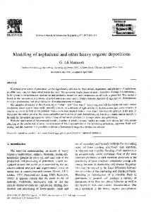
In the following section we compare the proposed strategy against a vehicle without torque vectoring in CarSim environment under two different scenarios: one assessing the understeer correction capabilities of the controller and another one assessing its ability to maintain the vehicle stability under quick steering inputs. For both scenarios we assume that no acceleration or braking commands come from the driver. 4.1 Step steer input scenario In the first scenario the vehicle is initially going straight and after 2s a step steer input of 10degs is applied on the wheels. The initial velocity is set to 16m/s (around 58km/h), which is 5m/s higher than the maximum allowable velocity for this steering input, and the road is assumed dry (µmax = 0.9). As we can see from Figure 2a, the vehicle using the MPC strategy achieves a much tighter trajectory, a direct result of the velocity regulation (Fig. 2b) achieved by controlling the torques on the front and rear axle (Figs 2e, 2f). It is also interesting to note from Figures 2c, 2d that for this scenario both the sideslip angle and yaw rate stay within the physical limits of the vehicle, as expressed by the sideslip angle and yaw rate constraints. 4.2 Double-lane change scenario In the second scenario we use the driver model available in CarSim to follow a quick double-lane change trajectory, as seen by the dotted line in Figure 3a. As we can see from Figure 3a, the vehicle without the front-to-rear torque vectoring capabilities becomes unstable towards the end of the manoeuvre due to the excessive sideslip angle and yaw rate values (Figs 3c, 3d) experienced by the vehicle. On the other hand, the vehicle using the MPC controller manages to stay stable by regulating the vehicle’s velocity (Fig. 3b) while at the same time constraining the vehicle’s sideslip angle (Fig. 3c) and yaw rate (Fig. 3d). This is however achieved by excessive oscillations on both the front and rear torque demands from the controller, as seen in Figures 3e, 3f a result of the somewhat limited torque vectoring capabilities inherent on such a vehicle topology.
5
CONCLUSIONS
A constrained optimal control strategy that uses combined velocity, yaw and sideslip regulation for stabilization of an electric vehicle with front-to-rear torque vectoring capabilities near the limit of lateral acceleration has been presented. The strategy is based on an MPC formulation which imposes constraints on the vehicle’s sideslip angle and yaw rate, along with the longitudinal slips on the front and rear axle. Despite the inherent limitations of such a vehicle topology, we have
(a) Trajectory of the two vehicles (MPC strategy in white) MPC Uncontrolled
56
Sideslip angle (deg)
Velocity (km/h)
54 52 50 48 46 44 42
50
6
40 30
4 2 0 −2 −4
MPC Uncontrolled Constraints
−6
40 38 0
8
Yaw rate (deg/s)
58
1
2
3
4
5 6 t (s)
7
8
9
−8 0
10
1
3
4
5 6 t (s)
7
400
400
300
300
200 100 0 −100 −200 −300 −400 0
8
9
10 0 −10 −20 MPC Uncontrolled Constraints
−30 −40 −50 0
10
1
2
(c) Sideslip angle
Rear axle torque (Nm)
Front axle torque (Nm)
(b) Velocity
2
20
3
4
5 6 t (s)
7
8
9
10
(d) Yaw rate
200 100 0 −100 −200 −300
1
2
3
4
5 6 t (s)
7
8
(e) Front axle torque
9
10
−400 0
1
2
3
4
5 6 t (s)
7
8
9
10
(f) Rear axle torque
Figure 2. Comparison of the MPC strategy and a vehicle without torque vectoring, along with the torques on the front and rear axle for the MPC strategy, for the step steer scenario.
shown that it is effective in correcting terminal understeer behaviour, while also stabilizing the vehicle under quick steering inputs. Based on the above results, the proposed controller will be next tested on a hardware-in-the-loop test rig, before implementing it on a prototype vehicle.
REFERENCES van Zanten, A. 2000. Bosch ESP Systems: 5 Years of Experience. SAE Technical Paper 2000-01-1633. Liebemann, E. & Fuehrer, D. 2007. More Safety with Vehicle Stability Control. SAE Technical Paper 2007-01-2759. Kang, J. & Kyongsu, Y. & Heo, H. 2012. Control Allocation based Optimal Torque Vectoring for 4WD Electric Vehicle. SAE Technical Paper 2012-01-0246.
(a) Trajectory of the two vehicles (MPC strategy in white) 6
MPC Uncontrolled
105
30
4 Sideslip angle (deg)
100 Velocity (km/h)
40
95 90 85 80 75 70
Yaw rate (deg/s)
110
2 0 −2
60 0
1
2
3
4
5 6 t (s)
7
8
9
−6 0
10
1
3
4
5 6 t (s)
7
MPC Uncontrolled Constraints
8
9
−40 0
10
1
2
(c) Sideslip angle
400
400
300
300
200 100 0 −100 −200 −300 −400 0
0 −10
−30
Rear axle torque (Nm)
Front axle torque (Nm)
(b) Velocity
2
10
−20
MPC Uncontrolled Constraints
−4
65
20
3
4
5 6 t (s)
7
8
9
10
(d) Yaw rate
200 100 0 −100 −200 −300
1
2
3
4
5 6 t (s)
7
8
(e) Front axle torque
9
10
−400 0
1
2
3
4
5 6 t (s)
7
8
9
10
(f) Rear axle torque
Figure 3. Comparison of the MPC strategy and a vehicle without torque vectoring, along with the torques on the front and rear axle for the MPC strategy, for the double-lane change scenario.
Siampis, E. & Massaro, M. & Velenis, E. 2013. Electric Rear Axle Torque Vectoring for Combined Yaw Stability and Velocity Control near the Limit of Handling. 2013 IEEE 52st Annual Conference on Decision and Control (CDC). Velenis, E. & Frazzoli, E. & Tsiotras, P. 2009. On steady-state cornering equilibria for wheeled vehicles with drift. 2009 IEEE 48th Annual Conference on Decision and Control (CDC). Piyabongkarn, D. & Lew, J.Y. & Rajamani, R. & Grogg, J.A. & Yuan, Q. 2007. On the use of torque-biasing systems for electronic stability control: Limitations and possibilities. IEEE Transactions on Control Systems Technology 15(3): 581589. Wheals, J.C. & Baker, H. & Ramsey, K. & Turner, W. 2004. Torque vectoring AWD driveline: Design, simulation, capabilities and control. SAE Technical Paper 2004-01-0863. Wheals, J.C. 2005. Torque vectoring driveline: SUV-based demonstrator and practical actuation technologies. SAE Technical Paper 2005-01-0553.
Wheals, J.C. & Deane, M. & Drury, S. & Griffith, G. 2006. Design and simulation of a torque vectoring rear axle. SAE Technical Paper 2006-01-0818. Garcia, C.E. & Prett, D.M. & Morari, M. 1989. Model predictive control: Theory and practice - A survey. Automatica 25(3): 335-348. Beal, C.E. & Gerdes, J.C. 2013. Model Predictive Control for Vehicle Stabilization at the Limits of Handling. IEEE Transactions on Control Systems Technology 21(4): 1258-1269. Gray, A & Ali, M. & Yiqi, G. & Hedrick, J.K. & Borrelli, F. 2012. Integrated threat assessment and control design for roadway departure avoidance. 15th International IEEE Conference on Intelligent Transportation Systems (ITSC). Falcone, P. & Ali, M. & Sjoberg, J. 2011. Predictive Threat Assessment via Reachability Analysis and Set Invariance Theory. IEEE Transactions on Intelligent Transportation Systems 12(4): 1352-1361. Bakker, E. & Nyborg, L. & Pacejka, H.B. 1987. Tyre Modelling for Use in Vehicle Dynamics Studies. SAE Technical Paper 870421. Maciejowski, J.M. 2002. Predictive control with constraints. Prentice Hall. Rajamani, R. 2012. Vehicle Dynamics and Control 2nd edition. Springer. Kienke, U. 2000. Automotive Control Systems. Springer. Gillespie, T.D. 1992. Fundamentals of Vehicle Dynamics. Society of Automotive Engineers SAE International. Antonov, S. & Fehn, A. & Kugi, A. 2011. Unscented Kalman filter for vehicle state estimation. Vehicle System Dynamics 49(9): 1497-1520.