Folkert Tangerman, Qiang Zhang. Department of Applied Mathematics and Statistics. State University of New York at Stony Brook. Stony Brook N.Y. 11794-3600.
Front Tracking in Two and Three Dimensions � James Glimm, Mary Jane Graham, John Grove, Xiao Lin Li, Todd Michael Smith, Dechun Tan, Folkert Tangerman, Qiang Zhang Department of Applied Mathematics and Statistics State University of New York at Stony Brook Stony Brook N.Y. 11794-3600 1
Introduction.
Front Tracking is the combination of two distinct computational traditions. Its purpose is to enable high quality, relatively coarse grid mesh solutions for problems complicated by the presence of fronts, interfaces, and other discontinuities, which may be of considerable geometric complexity. The rst of the two algorithmic ideas used in front tracking is upwind di�erencing, for uids, materials, and other conservation law based problems arising in physics. The second is computational geometry, from which we draw methods to represent, track, and process the geometric structures de ned by the discontinuities. This combination, which is called front tracking, is by now a mature capability in two dimensions [3], and has been used to achieve de nitive solutions to a number of problems which have otherwise resisted solution for decades. Here we report on recent extensions of front tracking to three dimensions [4], and we also present highlights from some recent two dimensional front tracking computations. Front Tracking applies to solutions which are conceptually piecewise smooth but not smooth. It thus applies to problems which contain important singularities, or jump discontinuities, concentrated on surfaces (curves in two dimensions). The location of the discontinuity surfaces are referred to as fronts. Front Tracking employs two grid systems. The traditional volume lling nite di�erence grid supports the smooth solution, located in the regions between the fronts, and a lower dimensional grid (the front, or interface) de nes the location of the discontinuity and the jump in the solution variables across it. The dynamics of the front comes from the mathematical theory of Riemann solutions, which is an idealized solution of a single jump Supported in part by the Applied Mathematics Subprogram of the U.S. Department of Energy DE-FG02-90ER25084, the Army Research O�ce, grant DAAL03-92-G-0185 and through the Mathematical Sciences Institute of Cornell University under subcontract to the State University of N.Y. at Stony Brook, ARO contract number DAAL-04-9510414, and the National Science Foundation, grant DMS-9500568 and DMS-9312098 �
1
discontinuity for a conservation law. Where surfaces intersect in lower dimensional objects (curves in three dimensions), the dynamics is de ned by a theory of higher dimensional Riemann problems, such as the theory of shock polars in gas dynamics. Nonlocal corrections to these idealized Riemann solutions provide the coupling between the solution values on these two grid systems. Modular programming allows both of the applications presented here and several others (elastic-plastic deformation and ow in porous media) to utilize the same geometry-based front tracking algorithms. The code is also modular with respect to the dimension of the ambient space, which is thus a run time or compile time variable, and is native parallel, for MIMD architectures. 2
Fluid Mixing.
We consider the problem of uid mixing resulting from the instability of an accelerated uid interface separating uids of di�erent densities. This process is known as the Rayleigh-Taylor (RT) problem in the case of steady acceleration, as by gravity, and the Richtmeyer-Meshkov (RM) instability in the case of impulsive acceleration, as by a shock wave. For both RT and RM mixing, Front Tracking solutions have been distinguished in their ability to compute mixing rates [6,10] in agreement with laboratory experiments [13,18]. These computations have been supported by theoretical analyses [1,7,17,21] which further validate the correctness of these computations. In these instabilities, the interface thickness is an important parameter, in determining the growth rate of the instability. The quality of Front Tracking computations lie in their absence of numerical di�usion at the interface, so that the computational interface better represents the experimental situation, in which physical di�usion at a molecular level is not an important phenomena.
2.1 Richtmeyer-Meshkov Instability
Richtmyer-Meshkov (RM) instability is a ngering instability between two di�erent
uids accelerated by a shock wave. When an incident shock collides with an interface between two di�erent materials, the material interface becomes unstable and small perturbations at the initial material interface grow. This interfacial instability was theoretically predicted by Richtmyer [14]. The rst experiment of this instability was performed by Meshkov [12]. The RichtmyerMeshkov instability plays an important role in studies of supernova and inertial con nement fusion. Richtmyer developed the linear theory for the case of re ected shock only. The linear theory for the case of re ected rarefaction wave can be found in [17]. In the same work [14], Richtmyer also proposed an impulsive model to simplify the dynamics of the RM unstable interface. The model approximates the incident shock as an impulse and the postshocked uids as incompressible. This impulsive model became a widely used theoretical model for RM instability. However, over thirty ve years of theoretical 2
studies, such linear theories failed to provide quantitatively correct predictions for the unstable growth of ngers at the material interface. Recently, Zhang and Sohn have developed nonlinear theories for RM instability in compressible uids [20]. The theories have no free parameters and provide analytical and quantitative predictions for the growth rates of the unstable ngers at the RM interface from early time linear growth stage to later time nonlinear growth stage, for compressible uids in two dimensions [21,22] and in three dimensions [19]. In Figure 1 we compare the predictions from the linear theory, the impulsive model and the nonlinear theory of Zhang and Sohn [21], as well as the result from full numerical simulations [8,10], for the growth rate and amplitude of the ngers at an air-SF 6 interface. A weak shock of Mach number 1.2 propagates from air to SF 6. The postshocked initial amplitude of the disturbance at the interface is a(0?) = 2:4mm and the postshocked Atwood number is A(0+) = 0:701. The wave length of the perturbation is 37.5mm and the pressure ahead of the shock is 0:8 bar. These parameters correspond to Benjamin's experiments on air-SF 6 interface. Figures 1(a) and 1(b) show that the predictions of the nonlinear theory are in remarkable agreement with the results from full numerical simulations, while the predictions of the linear theory for compressible uids and the linear impulsive model are qualitatively incorrect at later times. The experimental data is also shown in Figure 1(b). In experiments, it is di�cult to measure the growth rate directly. Instead, one measures the amplitude of the disturbed interfaces, then applies a linear regression analysis to determine a growth rate of the unstable interfaces. The growth rate determined from the experimental data was 9.2 m/s over the time period 310-750 �sec(see Figure 1b). Applying linear regression to the amplitude predicted by the nonlinear theory and to the amplitude obtained from the numerical simulations using front tracking method results in an identical 9.3 m/s for the growth rate as reported in [21] and [8]. Therefore, both the prediction of nonlinear theory and the results from front tracking are in excellent agreement with the experimental result. See [21,22] for further validation studies of the nonlinear theories.
2.2 Symmetry and Mesh Orientation
We also report on a di�erent, but very important, feature of front tracking. Because the front is locally aligned with the uid discontinuity, its computation is largely independent of mesh orientation e�ects. The e�ect of mesh orientation is a di�culty characteristic of nite di�erence schemes with xed rectangular grids. A nite di�erence grid can be thought of as a medium in which nonlinear uid waves propagate. For the regular rectangular grids often used in uid computations, the computed properties of the ow are not uniform in all directions but are usually favored in directions aligned with the grid. Front Tracking, however, utilizes a lower dimensional moving grid that follows the dynamical evolution of distinguished waves in the ow. This lower dimensional moving grid is referred to as the front and consists, in two dimensions, of a piecewise-linear system of curves which constitute an interface between di�erent regions of the ow eld. 3
Figure 1: Comparisons between the predictions of Growth Rate (a) and Amplitude (b) vs. Time for Richtmeyer-Meshkov instability by the linear theory, the impulsive model, and the nonlinear theory of Zhang and Sohn. The numerical simulation was performed by Holmes, et. al. using the two-dimensional front tracking code. In front tracking, these curves are propagated in the normal and tangential directions by an algorithm distinct from the scheme used to update the solution in the continuous regions. This results in a mesh which is locally aligned with the nonlinear waves being tracked. To illustrate the ability of Front Tracking to preserve symmetry, we consider a cylindrically symmetric Richtmyer-Meshkov problem. The RM problem is described generally in Section 2.1; we consider a perturbed circular material interface accelerated by a outgoing radial shock wave (See Figure 2(a)). In this case, the tracked waves are a contact discontinuity and a shock. Computational results in this problem show an unusual degree of symmetry and an absence of mesh orientation e�ects. In Figure 2(b) we see excellent symmetry, demonstrated in that even for instabilities with di�ering alignments with the underlying grid, the growth rates are approximately equal and the secondary structures are also in satisfactory agreement. 3
Etching and Deposition
The manufacture of semiconductor chips proceeds layer by layer with a succession of deposition and etching stages. There are variations on the basic processes, but they may all, as an approximation, be modeled as an evolving surface, whose dynamics is 4
Contact discontinuity
Transmitted shock
Contact
Reflected Rarefaction Trailing Edge
Shock
(a)
(b)
Figure 2: (a) Initial con guration for a cylindrically symmetric RM problem. A circular shock is shown before impinging on a density discontinuity which has an initial harmonic perturbation. The computation was performed on a 200x200 grid. (b) Late stage of RM problem. The incident shock has completed the refraction process, resulting in an inward re ected wave, a de ected material interface and an outward moving transmitted shock. Note the symmetry of the individual ngers. given by a Hamilton-Jacobi equation [15] St + H (SX ) = 0 (3.1) for a function S (X; t) de ned on R3 whose level set S = 0 describes the evolving surface of the chip. SX denotes the gradient of S . The Hamiltonian (or ux function) H usually has an additional spatial dependence indicating varying material properties or varying position with respect to an ion beam, which we ignore for the purpose of this paper. The semiconductor manufacturing industry has various codes for studying the two dimensional problem: the evolution of cross-sections of trenches. For instance, a front tracking algorithm for moving curves in R2 has been constructed by [9]. A proper understanding of three dimensional e�ects is important for the analysis and design of the manufacturing process and is our motivation to contribute to the development of a simulation code. The Hamiltonians of interest have the form: H (P ) = c(P=jjP jj) jjP jj (3.2) for jjP jj 6= 0 where c is a smooth (C 2) function on the unit sphere. The function c is known as the etching or deposition e�ciency. An example is given by constant c, as is the case for chemical vapor deposition (CVD) or low energy etching. For high energy etching, c usually has a non-trivial dependence on surface angle with respect to the incoming beam. 5
Solutions to the Hamilton-Jacobi equation (3.1) are not unique, a phenomenon associated with the existence of caustics. However existence and uniqueness holds within a subclass of weak solutions: viscosity solutions [2,11]. Volume based approaches [16] to solve (3.1) have di�culty near corners and edges in the level surface, where they require ne meshing. The front tracking approach to this problem is surface based: we only mesh the object of interest, the moving surface. We replace the use of ne grids near surface discontinuities by the solution of an analytic problem. In this manner we can use quite coarse grids for a desired accuracy. As time evolves we regrid the surface. This use of coarse grids is a considerable improvement in the utilization of computational resources, but requires a larger investment in theoretical resources: the solution of analytic problems and e�cient regridding strategies. We describe our front tracking methodology in more detail and present numerical results.
3.1 Propagation and Riemann Problems
The evolving level set is mathematically represented as a two dimensional interface: smooth surfaces, stitched together along curves (edges or cusps) which meet at nodes (corners). Requiring such an interface to be a level set of a viscosity solution, admissible in our terminology, implies Hamiltonian dependent constraints on the geometry at curves and nodes [5]. The main concern is then the admissible propagation of the interface. If the initial interface is not admissible it must bifurcate into an admissible one: for instance a curve may be inadmissible, thus necessitating its removal or replacement by a number of curves. Front tracking require rules for propagating surface points, curve points, and nodes. The propagation is based on a nite di�erence approximation to the characteristic equation. Rules have to be consistent and are usually quite generic for surface points and most complicated and physics dependent for curve points and nodes. In order to use coarse grids correctly near interface discontinuities we need to understand the propagation of idealized geometries: Riemann problems. Consider a point X0, the origin for convenience, in the interface at some time t, t = 0 for convenience. Near X0 = 0 we seek the solution S (X; t) in the form: S (X; t) = t � Z ( Xt ) Since (rS )(X; t) = (rZ )(X=t), and since S (X; 0) near X = X0 = 0 is given, (rZ ) is given at the sphere at in nity ( X0 ). If we can determine Z , then for t small, S (X; t) is determined near X = X0. Denoting the velocity Xt by V , we obtain as equation for Z : Z (V ) ? V � (rZ )(V ) + H ((rZ )(V )) = 0 (3.3) which is also referred to as a Hamilton-Jacobi equation, and which has a parallel theory of viscosity solutions [2,11]. One needs to construct an admissible level set Z = 0 subject to the boundary conditions on the sphere at in nity imposed by the interface geometry at X0. As shown in [5,2,11] a unique admissible Lipschitz solution exists and therefore, at least in theory, the matter of propagation and bifurcation is resolved. The main 6
ingredient to our front tracking method is the explicit construction of the solution in the cases of at hand. The propagation algorithm is simplest when the initial interface is admissible everywhere, i.e. bifurcation is not required. Surface Points: Let X be a surface point with unit normal P . The Riemann problem has only one solution: Z (V ) = P � V ? H (P ). Since there is no discontinuity to track we have a single constraint on the velocity V at the point X , namely Z (V ) = 0 or: P � V = H (P ), which speci es the normal component of V . Curve Points: (Shocks) At a curve point X the tangent directions to the interface consists of two hyperplanes, with normals P0 and P1. For a vector a tangent to the curve at X we must have: P0 � a = P1 � a. If X is an admissible curve point Z is of the form Z = P0 � V ? H (P0) on one side and of the form Z = P1 � V ? H (P1) on the other. Since we want to track the curve, we choose the velocity V , so that Z (V ) = 0 which leads to two equations: Pi � V ? H (Pi ) = 0, i = 0; 1. Node Points: A typical case is a triple point: where three planes, with normals P0, P1 and P2 meet. Admissibility and bifurcations for a triple point is completely resolved [5]. In the admissible case, the triple point propagates as a triple point and its velocity V is determined by: Pi � V ? H (Pi ) = 0, i = 0; 1; 2.
3.2 Example
As a rst approximation one may take the etch rate c as a function of angle between surface normal and the direction of the ion beam. Although at rst glance one might expect the etch rate to be largest when this angle is 0 radians and to decrease monotonically as this angle varies from 0 to �2 radians, this is not necessarily the case. Under most circumstances the largest etch rate is obtained at a non zero angle and the graph of c as a function of � = (P; beam) can be as in Figure 3.2. In the 6
c Θ
Figure 3: Shape of etch rate c for � between ? �2 and
� 2
example we present, c has that form c(�) = 5 cos2 � ? 4 cos4 �. The initial geometry is a square hole in a horizontal plane which the ion beam enters vertically. This initial geometry has four curves at the bottom, four vertical curves and four curves along the rim as well as four nodes at the bottom and four 7
Inside Top of Hole (t = 0)
Inside Top of Hole (t > 0)
Inside Bottom of Hole (t = 0)
Inside Bottom of Hole (t > 0)
Figure 4: Riemann solutions for the node types in a square hole along the top. The etch rate in our example is zero on the vertical sides and positive on the horizontal sides. In Figure 4 we graphically represent of the solution of the Riemann problems for the two types of nodes. Near the rim the geometry bifurcates into two systems of curves: a copy of the original geometry which moves down vertically and a closed curve, rounded in the vicinity of corners of the initial condition, which moves into (and with) the horizontal plane. Together they span a beveled surface, conically shaped near the corners. Near the bottom, the geometry also changes, albeit it less drastically. The perfectly vertical sides in the initial condition turn into surfaces which have a shock where they meet the bottom plane under an angle of less than �2 radians, and steepen to become vertical, where no etching takes place. These surfaces meet at a shock. In our computation we then track thirteen curves, one of which is closed, and eight nodes with non trivial Riemann problems for each. 8
Figure 5: Shown are, on the left, the initial interface and, on the right, the propagated interface. In order to initialize this geometry we constructed as initial condition an approximation to the bifurcation. Figure 5 shows on the left a side view of this initial condition. This approximation has sharp corners along the rim, a poor approximation to a smoothly rounded curve; the sides of the hole are not quite vertical at the bottom. No further geometric bifurcations take place during the numerical experiment. The right part of Figure 5 shows the propagated interface from the same vantage point. Etching has clearly occurred: the propagated interface is deeper and wider than the initial interface. Also one can clearly discern that the beveled interface at the rim has rounded signi cantly in the corners. References
[1] Y. Chen, Y. Deng, J. Glimm, G. Li, D. H. Sharp and Q. Zhang, A Renormalization Group Scaling Analysis For Compressible Two-Phase Flow, Phys. Fluids A, 5 (1993), pp. 2929{2937. [2] M. G. Crandall, L. C. Evans and P. L. Lions, Some Properties of Viscosity Solutions of Hamilton-Jacobi equations, Trans. Amer. Math. Soc., 282 (1984), pp. 487{502. [3] J. Glimm, Nonlinear and Stochastic Phenomena: The Grand Challenge for Partial Di�erential Equations, SIAM Rev., 33 (1991), pp. 626{643. [4] J. Glimm, J. W. Grove, X. L. Li, K. -M. Shyue, Q. Zhang and Y. Zeng, Three Dimensional Front Tracking, 1995, Report No. SUNYSB-AMS-95-17. [5] J. Glimm, H. Kranzer, D. Tan, F. Tangerman and G. Vanderwoude, Wave Fronts in Deposition and Etching Processes, To appear, 1996.
9
[6] J. Glimm, X. L. Li, R. Menikoff, D. H. Sharp and Q. Zhang, A Numerical Study of Bubble Interactions in Rayleigh-Taylor Instability for Compressible Fluids, Phys. Fluids A, 2 (1990), pp. 2046{2054. [7] J. Glimm, D. Saltz and D. H. Sharp, Renormalization Group Solution of Two-Phase Flow Equations for Rayleigh-Taylor Mixing, University at Stony Brook Preprint No. SUNYSB-AMS-95-15, 1995, submitted Phys. Rev. Lett.. [8] J. Grove, R. Holmes, D. H. Sharp, Y. Yang and Q. Zhang, Quantitative Theory of Richtmyer-Meshkov Instability, Phys. Rev. Lett., 71 (1993), pp. 3473{ 3476. [9] S. Hamaguchi, M. Dalvie, R. T. Farouki and S. Sethuraman, A Shocktracking Algorithm for Surface Evolution under Reactive-ion Etching, J. Appl. Phys, 74(8) (1993), pp. 5172{84. [10] R. L. Holmes, J. W. Grove and D. H. Sharp, Numerical Investigation of Richtmyer-Meshkov Instability Using Front Tracking, J. Fluid Mech., 301 (1995), pp. 51{64. [11] P. L. Lions, Generalized Solutions of Hamilton-Jacobi Equations, Pitman, Research Notes in Mathematics, 69, Boston-London-Melbourne, 1982. [12] E. E. Meshkov, Instability of a shock wave accelerated interface between two gases, NASA Tech. Trans., F-13 (1970), p. 074. [13] K. I. Read, Experimental Investigation of Turbulent Mixing by Rayleigh-Taylor Instability, Physica D, 12 (1984), p. 45. [14] R. D. Richtmyer, Taylor Instability in Shock Acceleration of Compressible Fluids, Comm. Pure Appl. Math., 13 (1960), pp. 297{319. [15] D. S. Ross, Ion Etching: An Application of the Mathematical Theory of Hyperbolic Conservation Laws, J. Electrochem. Soc: Solid-State Science and Technology, 135 (1988), pp. 1235{1240. [16] J. A. Sethian and D. Adalsteinsson, An Overview of Level Set Methods for Etching, Deposition, and Lithography Development, University of California, Berkeley, preprint, 1996. [17] Y. Yang, Q. Zhang and D. H. Sharp, Small Amplitude Theory of RichtmyerMeshkov Instability, Phys. Fluids, 6 (1994), pp. 1856{1873. [18] D. L. Youngs, Numerical Simulation of Turbulent Mixing by Rayleigh-Taylor Instability, Physica D, 12 (1984), pp. 32{44. [19] Q. Zhang and S. Sohn, Quantitative Theory of Richtmyer-Meshkov Instability in Three Dimensions, State Univ. of New York at Stony Brook, Report No. SUNYSB-AMS-96-11, 1996. [20] , Nonlinear Solutions of Unstable Fluid Mixing Driven by Impulsive Force, State Univ. of New York at Stony Brook, Report No. SUNYSB-AMS-96-09, 1996. [21] , An Analytical Nonlinear Theory of Richtmyer-Meshkov Instability, Phys. Lett. A, 212, (1996), p. 149. [22] , Spike and Bubble Dynamics in Richtmyer-Meshkov Instability, State Univ. of New York at Stony Brook, Report No. SUNYSB-AMS-96-10, 1996. 10