Approximation of 2D Function Using Simplest Neural Networks- A Comparative Study and Development of GUI System Tarun Varshney, Student Member, IEEE, and Satya Sheel, Senior Member, IEEE
Abstract--This
paper demonstrates the function approximation capability of feed forward neural network (FFNN). An attempt has been made to develop the Graphical user Interface (GUI) system for function approximation. This GUI system can handle the function approximation of any nonlinear/linear function which can have any number of input variable and 6 output variables. Parameters of neural network can be set from a single panel. This GUI system provides approximation for various functions which made this GUI universal for the wide range of the users without theoretical knowledge about the function approximation. A Neural network with a single hidden layer has been used to approximate the functions. To train the neural network various type of learning algorithms has been accumulated in GUI system. Two 2-D benchmark problem has been tested. Finally comparison has been made which shows that Levenberg-Marquardt (LM) back propagation with single hidden layer FFNN converges faster than other training algorithms. Index Terms--Function approximation, GUI, LevenbergMarquardt Algorithm ,multilayer neural network, MISO.
I. INTRODUCTION
F
unction approximation is a significant task in numerous engineering applications ranging from dynamic system identification to control, fault detection, optimization and classification. It refers to curve fitting equations (i.e., function approximators) to observed data. The term function approximator is used to represent multivariable approximation models, mostly nonlinear, which possess a number of adjustable parameters known as weights. Common approximation methods include least squares fit, neural networks in the form of feed forward multilayer perceptrons (MLPs) ,radial basis function (RBF) networks [2] etc. Neural networks are a convenient means of representation because they are universal approximators that can learn data by example [8], [14] or reinforcement [9], either in batch or sequential mode. Typically, training involves the numerical optimization of the error between the data and the actual network’s performance with respect to its adjustable Tarun Varshney is with Department of Electronic & Instrumentation Engg., MIT, Moradabad, UP, INDIA (e-mail:
[email protected]). Satya Sheel is with the Department of Electrical Engineering, MNNIT, Allahabad,UP, INDIA (e-mail:
[email protected]).
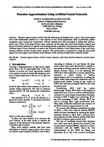
parameters or weights. Considerable effort has gone into developing techniques for accelerating the convergence of these optimization-based training algorithms [10]–[13], [17][20]. An alternative to the multilayer perceptron is the Radial Basis Function (RBF) network. [15] Proved theoretically that the RBF type neural networks are capable of universal approximations and learning without local minima, thereby guaranteeing convergence to globally optimum parameters. Generally, the traditional radial basis function neural network may sometimes be considered prohibitively expensive to implement in computational terms for large amounts of training data [15], [16]. The performance of a trained RBF network depends on the number and locations of the radial basis functions, their shape and the method used for learning the input-output mapping. The most popular existing learning strategies for RBF neural networks can be classified as follows: (i) strategies selecting the RBF centers randomly from the training data, (ii) strategies employing unsupervised procedures for selecting the RBF centers, and (iii) strategies employing supervised procedures for selecting the RBF centers. Two difficulties are involved with traditional RBF networks: the initial configuration of an RBF network needs to be determined by a trial-and-error method, and the performance suffers degradation when the desired locations of the center of the RBF are not suitable. In this paper a GUI system for function approximation using neural network with single hidden layer has been modeled where user can configure the various parameters of neural network. This paper is organize as follows- Section II describes the various features of GUI system, the basics of LM algorithm are illustrated in section III , results of simulation and comparisons has been shown in section IV and finally concluding remarks are given in section V. II. DEVELOPMENT OF GUI SYSTEM To simplify the simulation procedure a GUI system has been developed and shown in Fig. 1. The various simulation parameters can be set from a single panel. User may choose any number of hidden neurons for hidden layer. Network training can be stopped by examining either maximum number of iteration/epochs or permissible error whichever is met first. One can choose learning rate and momentum rate
978-1-4244-8542-0/10/$26.00 ©2010 IEEE
2
between 0 to1. This GUI system handles any numbers of input variable and maximum six (06) output variables. The efficiency of neural network training improves by normalizing the inputs and outputs data. Normalization of input & output data pair can be done between -1 to 1 as well as for 0 and standard mean of 1. Input and output pairs has to be store in an excel file and can be fetch by typing the name of file in the field of filename.xls. Activation function for hidden layer and output layer can be chosen e.g sigmoid, log sigmoid, linear. To train the neural network a variant of backpropagation algorithm can be opt from following list Gradient descent backpropagation Gradient descent with momentum backpropagation Gradient descent with adaptive learning rate backpropagation Gradient descent with momentum and adaptive learning rate backpropagation Levenberg-Marquardt backpropagation BFGS Quasi-Newton backpropagation RPROP backpropagation Bayesian Regulation backpropagation Conjugate gradient backpropagation with Polak-Ribiere updates Conjugate gradient backpropagation with FletcherReeves updates Conjugate gradient backpropagation with Powell-Beale restarts Scaled conjugate gradient backpropagation Conjugate gradient backpropagation with Powell-Beale restarts One step secant backpropagation. Although this GUI system has been tested for various nonlinear functions but in this paper only the results of two nonlinear functions has been reported. It has been found that LM algorithm converges faster than other training algorithms, a brief overview of LM algorithm is described in next section. III. LM TRAINING ALGORITHM LM algorithm is the blend of steepest descent and the Gauss-Newton searching methods and illustrated in [5] - [6]. It consists from the following equation:
JT J
I
JT E
(1)
Where J is the Jacobian matrix for the system, λ is the Levenberg's damping factor, δ is the weight update vector and E is the error vector containing the output errors for each input vector used on training the network. The λ damping factor is adjusted at each iteration, and guides the minimization process. This adjustment for λ is done by using an adjustment factor v, usually defined as 10. If λ needs to increase, it is multiplied by v. If it needs to decrease, then it is divided by v. The process is repeated
until the error decreases. When this happens, the current iteration ends. The following steps are involved in LM algorithm; 1. Compute the Jacobian of the system T
2. Compute the error gradient g J E 3. Solve (H + λI)δ = g to find δ 4. Update the network weights w using δ 5. Recalculate the sum of squared errors using the updated weights 6. If the sum of squared errors has not decreased, Discard the new weights, increase λ using v and go to step 3. 7. Else decrease λ using v and stop. IV. SIMULATION RESULTS AND DISCUSSION Single hidden layer neural network has been considered because it has been well proven that single layer neural networks are universal approximators. Two benchmark problems are tested with this GUI system. For both cases 1000 pairs of input and output has been generated. This set of data has been divided into training, testing and validation data sets. 60 % data has been used to train the neural network and 20 % data has been used for testing and rest data set has been used for validation purpose. Once input output pairs are generated, it must be preprocessed otherwise, the neural network will not produce correct output. For preprocessing normalization has been done between -1 to +1. Neural network has been trained for 0.001 performance goal. In each problem the neural network is trained from any arbitrarily random weight initialization. A. Two dimensional function-I The 2-D Gabor function is given by following equation
g ( x1 , x2 ) =
1 e 2 (0.5) 2
[( x12 x22 ) / 2(0.5)2 ]
cos(2 ( x1 x2 )) (2)
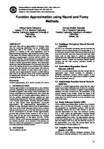
where x1 and x2 are input variables as in [3]. For this case 1000 data are generated in the range of [-0.5 0.5]. The neural network has been trained with LM algorithm. Learning rate and momentum coefficient has been chosen 0.5 and 0.9 respectively. Simulation has been carried out with the consideration of 15 hidden neurons in hidden layer. By the observation Fig. 2 it can be seen that feed forward neural network with single hidden layer can approximate the 2-D Gabor function which is highly nonlinear. The data set is divided into three distinct sets called training, testing and validation sets. Training set is largest set and used by neural network to learn patterns presents in data. The testing set is used to evaluate the generalization ability of a trained network. A final check on a performance of the trained network is made using validation set. The comparison of square error for all three sets with respect to epochs has been
3
Fig. 1. Overlook of GUI system
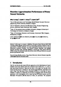
shown in Fig. 3 and it has been noticed that only in 199 epochs neural network is able to get performance goal. The RBF neural network has been used to approximate the Gabor function [3]. The simulation results of present work have been compared in Table 1. From the observation it is clear
that Feed forward neural network with single hidden layer can better approximate the 2-D Gabor function. B. Two dimensional function-II In this case a nonlinear function is approximated which is given as
TABLE 1 PERFORMANCE COMPARISON FOR GABOR FUNCTION
g ( x, y ) SN
1 2 3 4 5
Algo
BP BP LF-I LF-II LM
Type of Network
No. of centers
RBF RBF RBF RBF FFNN
40 80 40 40 ---
No. of hidden neurons ------------15
rms error
0.0847241 0.0314169 0.0192033 0.0186757 0.001
sin(20 x 2 20 x
2
y2 ) 1 cos(10 x 2 2 5 y
y2 )
(3)
where x and y are input variables as in [4]. Simulation has been carried out with the same simulation environment of that [4] except in place of 40 hidden neurons, 15 neurons have been chosen in hidden layer. LM algorithm has been selected to train the neural network. Learning rate and momentum coefficient has been chosen 0.01 and 0.8 respectively. Fig. 4 shows that neural network with the architecture of 2-15-1 can approximate the function which is given by Eq. 3. From the comparison graph Fig. 5 it is observed that only in 37 epochs neural network is able to get performance goal of 0.001. Table2 concludes that the LM algorithm can approximate the non linear function much faster than the gradient descent with momentum constant. It takes 87.66% lesser epochs to approximate the function with the performance goal of 0.001. It is worth to mention that rather than 40 neurons only 15 neurons are sufficient to approximate the function with LM algorithm. With the lesser number of hidden neurons computation time can be saved.
Fig. 2. Function-I (Gabor function) approximation by neural network
Fig. 4. Function-II approximation by neural network Fig. 3. Comparisons of performance for function-I
y 0.3 2
4 [9]
[10]
[11]
[12]
[13] [14] Fig. 5. Comparisons of performance for function-II [15]
TABLE 2 PERFORMANCE COMPARISON FOR SECOND FUNCTION S N 1 2
Algorithm BP with momentum LevenbergMarquardt
Structure of NNs 2-40-1
Momentum term 0.80
Learning rate 0.01
Epochs
2-15-1
0.80
0.01
37
300
This paper presents GUI system to approximate the functions using neural network. This GUI provides computing without the deepest theoretical knowledge which is the main advantage of this system. User can change configuration, and the most of the important parameters of the neural network. This contribution shows the function approximation capability of feed forward neural network with single hidden layer. Two 2-D highly non linear functions are tested where LM algorithm has been chosen for training. Simulation results confirmed that FFNN with single hidden layer having 15 neurons have better function approximation capability than the radial basis function and LM algorithm converges faster than back propagation algorithm with momentum constant. VI. REFERENCES [2]
[3]
[4] [5] [6] [7] [8]
[17]
[18]
V. CONCLUSIONS
[1]
[16]
S. Haykin, Neural Networks: A Comprehensive Foundation. Englewood Cliffs, NJ: Prentice-Hall, 1999. Handbook of Intelligent Control, D. A. White and D. A. Sofge, Eds., Van Nostrand, New York, 1992, pp. 65–86. P. J. Werbos, Neurocontrol and Supervised Learning: An Overview and Evaluation. Yinyin Liu, Janusz A. Starzyk, and Zhen Zhu, “Optimized Approximation Algorithm in Neural Networks Without Overfitting,” IEEE transactions on neural networks, vol. 19, no. 6, June 2008. R. S. Sutton and A. G. Barto, Reinforcement Learning. Cambridge, MA: MIT Press, 1998. D. E. Rumelhart, G. E. Inton, and R. J.Williams, “Learning representations by back-propagating errors,” Nature, vol. 323, pp. 533–536, 1986. R. A. Jacobs, “Increased rates of convergence through learning rate adaptation,” Neural Netw., vol. 1, no. 4, pp. 295–308, 1988. K. Rigler, J. M. Irvine, and T. P. Vogl, “Rescaling of variables in backpropagation learning,” Neural Netw., vol. 3, no. 5, pp. 561–573, 1990. Toledo, M. Pinzolas, J. J. Ibarrola, and G. Lera, “Improvement of the neighborhood based Levenberg–Marquardt algorithm by local adaptation of the learning coefficient,” IEEE transactions on neural networks, vol. 16, no. 4, July 2005.
Magoulas, G.D.; Plagianakos, V.P.; Vrahatis, M.N., “Development and convergence analysis of training algorithm with local learning rate adaptation,” International Joint Conference on Neural Networks, pp 21 - 26 vol.1, 2000. Yong Li; Yang Fu; Hui Li; Si-Wen Zhang; “The improved training algorithm of back propagation neural network with self-adaptive ,” International Conference on Computational Intelligence and Natural Computing, pp. 73 – 76, 2009. Chien-Cheng Yu; Bin-Da Liu, “A back propagation algorithm with adaptive learning rate and momentum coefficient,” International Joint Conference on Neural Networks, pp. 1218 – 1223, 2002 Sheel, S.; Varshney, T.; Varshney, R., “Accelerated learning in MLP using adaptive learning rate with momentum coefficient,” International Conference on Industrial and Information Systems, pp. 307 – 310, 2007. J. Park,I. W. Sandberg, “Universal approximation networks,” Neural Computation 3, pp 246-257, 1991. Shenmin Song, Zhigang Yu, Xinglin Chen, “A novel radial basis function neural approximation,” International Journal of Information Technology, vol. 11 No.9 , 2005. Martin T.Hagan & Mohammad B.Menhaj , “Training feed forward networks with the Marquradt algorithm,” IEEE transactions on neural networks, vol. 5, no. 6.,1994 Wilamowski, B.M., Cotton, N., Hewlett, J. & Kaynak, O., “Neural network trainer with second order learning algorithms,” International Conference on Inteligent engineering systems, pp 127 – 132, 2007. Laxmidhar Behera, “On adaptive learning rate that guarantees convergence in feed forward networks,” IEEE transactions on neural networks, Vol. 17 no.5, pp 1116 – 1125, 2006. Weishui Wan, “Implementing online natural gradient learning: problem and solutions, IEEE transaction on neural networks, Volume 17, No. 2, pp 317- 329, 2006.