sound-delivery tubes sealed into the acoustic meati (Sokolich, US. Patent 4 .... Open triangles mark the bandwidth used for the determination of Q 1~ dB. Closed ...
JOURNALOFNEUROPHYSIOLOGY Vol. 64, No. 5, November
1990.
Printed
in U.S.A.
Functional Topography of Cat Primary Auditory Cortex: Distribution of Integrated Excitation CHRISTOPH E. SCHREINER AND JULIE R. MENDELSON Coleman Laboratory, Department of Otolaryngology, University of California, San Francisco, California 94143-0732 SUMMARY
AND
INTRODUCTION
CONCLUSIONS
1. Neuronal responses to tones and transient stimuli were mapped with microelectrodes in the primary auditory cortex (AI) of barbiturate anesthetized cats. Most of the dorsoventral extent of AI was mapped with multiple-unit recordings in the high-frequency domain (between 5.8 and 26.3 kHz) of all six studied cases.The spatial distributions of I) sharpness of tuning measured with pure tones and 2) response magnitudes to a broadband transient were determined in each of three intensively studied cases. 2. The sharpness of tuning of integrated cluster responses was defined 10 dB above threshold (Qlo dB, integrated excitatory bandwidth). The spatial reconstructions revealed a frequency-independent maximum located near the center of the dorsoventral extent of AI. The sharpness of tuning gradually decreased toward the dorsal and ventral border of AI in all three cases. 3. The sharpness of tuning 40 dB above response threshold was also analyzed (Q 4~dB). The Q40dBvalues were less than one-half of the corresponding Q10 dBvalue. The spatial distribution showed a maximum in the center of AI, similar to the Qlo dBdistribution. In two out of three cases, restricted additional maxima were recorded dorsal to the main maximum. Overall, Qlo dBand Q40 dB were only moderately correlated, indicating that the integrated excitatory bandwidth at higher stimulus levels can be influenced by additional mechanisms that are not active at lower levels. 4. The magnitude of excitatory responses to a broadband transient (frequency-step response) was determined. The normalized response magnitude varied between < 1% and up to 100% relative to a characteristic frequency (CF) tone response. The step-response magnitude showed a systematic spatial distribution. An area dorsal to the Q 1odBmaximum consistently showed the largest response magnitude surrounded by areas of lower responsivity. A second spatially more restricted maximum was recorded in the ventral-third of each map. Areas with high-transient responsiveness coincided with areas of broad integrated excitatory bandwidth at comparable stimulus levels. 5. The distribution of excitation produced by narrowband and broadband signals suggest that there exists a clear functional organization in the isofrequency domain of AI that is orthogonal to the main cochleotopic organization of the AI. Systematic spatial variations of the integrated excitatory bandwidth reflect underlying cortical processing capacities that may contribute to a parallel analysis of spectral complexity, e.g., spectral shape and contrast, at any given frequency. 6. Similarities and consistencies in the spatial distribution of responses to narrowband and broadband signals indicate that the integrated excitatory bandwidth, as determined with the multiple-unit technique, is a useful tool to explore global functional properties of AI. It is suggestive that systematic changes in 1) the convergence of the projections to the cortical locations and 2) the extent of inhibitory influences are mainly responsible for the functional organization described along the isofrequency domain.
1442
0022-3077/90
$1 SO Copyright
One of the fundamental organizational principles in the mammalian forebrain is the topographic representation of the sensory epithelium. Such a topographic organization has been demonstrated for a number of auditory cortical fields, including the primary auditory field (AI) (Knight 1977; Merzenich et al. 1975; Reale and Imig 1980; Woolsey and Walzl 1942). Although the sensory epithelium of the auditory system is one-dimensional, a row of receptor cells along the basilar membrane in the cochlea, the topographic representation of the receptor surface, occupies two spatial dimensions in AI in addition to the cortical depth. Extensive multiple-unit mapping studies of AI in the cat (Merzenich et al. 1975; Reale and Imig 1980) have shown a strict cochleotopic representation along its caudal/rostral dimension. This organization is expressed as an increase in the characteristic frequency (CF) of neuronal frequency tuning curves (FTCs) from low CFs in the caudal aspect of AI to progressively higher CFs toward the rostra1 border of AI. In the spatial dimension orthogonal to the cochleotopic frequency gradient of AI, i.e., in its dorsoventral extent, no clearly expressed gradient of CF has been observed. It was concluded that cortical neurons with similar CFs are arranged along “isofrequency contours” oriented along the dorsal-to-ventral extent of AI. The first evidence for a spatial segregation of functional parameters along the “isofrequency domain” came from the discovery of “binaural interaction bands” that transect isofrequency contours in AI (Imig and Adrian 1977; Middlebrooks et al. 1980). The isofrequency domain of AI then consists of alternating patches of neurons that differ in their binaural integration of excitatory or inhibitory inputs and in their thalamic and cortical sources of input (Imig and Brugge 1978; Imig and Reale 198 1; Middlebrooks and Zook 1983). The spatial distributions of other functionally significant response characteristics of neurons in the isofrequency domain of AI have not been extensively studied. However, a multiple-unit study of the secondary auditory field (AII) that included ventral aspects of AI (Schreiner and Cynader 1984) indicated a systematic spatial variation of another important functional parameter in ventral AIthe sharpness of tuning. More extensive analyses of isofrequency-domain representations have been conducted in the auditory cortex of echolocating bats. Several topographic representations of functionally significant parameters relating to biosonar orientation sounds have been demonstrated (e.g., Suga 1965, 1984; Suga and Manabe 1982). By contrast, no clear func-
0 1990 The American Physiological Society
ISOFREQUENCY
DOMAIN
OF AI: INTEGRATED
tionally identified specialization of auditory cortical fields has been described in other mammalian species. To address the issue of cortical-field organization and specificity in signal processing, an important question in auditory neurobiology is what functional parameters are represented in the extended “isofrequency dimension” of auditory cortical areas. The goal of this study was to examine, in more detail, the spatial distribution of some response features of potential functional significance in the isofrequency domain of the high-frequency region in the AI of anesthetized cats. In this initial report the spatial distribution of excitatory neuronal activity in response to pure tones and broadband transients is presented. Cortical maps for sharpness of tuning 10 and 40 dB above response threshold as well as the spatial distribution of response magnitude to a transient signal will be illustrated and compared. Reports will follow that address stimulus-intensity effects and responses to frequency sweeps in the same animals. METHODS
Surgical preparation Results presented in this report were obtained in the right hemispheres of adult cats. Anesthesia was induced with an intramuscular injection of ketamine hydrochloride ( 10 mg/kg) and acetylpromazine maleate (0.10 mg/kg). After venous cannulation, an initial dose of pentobarbital sodium (30 mg/kg) was administered. Animals were maintained at a surgical level of anesthesia with a continuous infusion of pentobarbital sodium (2 mg . kg-’ h-‘) in lactated Ringer solution (infusion volume, 3.5 ml/h) and, if necessary, with supplementary intravenous injections of pentobarbital sodium. The cats were also given dexamethasone sodium phosphate (0.14 mg/kg im) to prevent brain edema and atropine (1 mg im) to reduce salivation. The temperature of the animals was monitored with a rectal probe and maintained at 37.5”C by means of a heated water blanket with feedback control. The head was fixed, leaving the external meati unobstructed. The temporal muscle on the right hemisphere was then retracted and the lateral cortex exposed by a craniotomy. The dura overlying the middle ectosylvian gyrus was removed, the exposed cortex covered with silicone oil, and a photograph of the surface vasculature was taken to record the electrode penetration sites. l
Stimulus generation and delivery Experiments were conducted in a sound-shielded room (IAC). Auditory stimuli were presented via calibrated headphones (STAX 54) enclosed in small chambers that were connected to sound-delivery tubes sealed into the acoustic meati (Sokolich, US Patent 4,25 1,686; 198 1). The sound-delivery system was calibrated with a sound-level meter (Briiel & Kjaer 2209) and a waveform analyzer (General Radio 152 1-B). The frequency response of the system was essentially flat up to 12 kHz and did not have major resonances deviating more than 6 dB from the average level. Above 15 kHz, the output rolled off at a rate of 10 dB/octave. Tones were generated by a microprocessor (TMS320 10; 16-bit D/A converter at 120 kHz; low-pass filtered at 35 kHz). The processor-related useful dynamic range of these stimuli was ~78 dB, allowing a 3-bit amplitude resolution at the lowest-applied stimulus level. Additional attentuation was provided by a pair of passive attenuators (HP). The duration of the tone bursts was 50 ms including 3 ms rise-fall time. The interstimulus interval was 500- 1,000 ms.
EXCITATION
1443
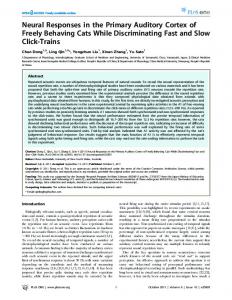
For each recording site responses were recorded to at least 675 different tone bursts. Tone bursts were presented in a pseudorandom sequence of different frequency-level combinations selected from 15 level values and 45 frequency values. From the responses to all stimuli, frequency-response areas (FRAs) were reconstructed. The minimum step between stimulus levels was 5 dB, resulting in a dynamic range of 75 dB for the FRA. The frequency range covered by the 45 frequency steps was geometrically centered around the estimated CF of the recording site and covered between 2 and 4 octaves, depending on the estimated width of the FRA. Stimulus frequencies were equidistant on a logarithmic frequency scale. A frequency step generated with a Wavetek 185 was used to produce a broadband transient signal. The frequency changed from 250 Hz to 64 kHz, or vice versa, within ~20 ps. The electric input and acoustic output spectra of the speaker system for the frequency step are shown in Fig. 1.
Recording procedure Parylene-insulated tungsten microelectrodes with impedances at 1 kHz of 0.8-l .3 MQ were introduced into the auditory cortex with a hydraulic microdrive (KOPF) remotely controlled by a stepping motor. All penetrations were roughly orthogonal to the brain surface. The recordings reported here were derived at an intracortical depth ranging from 600 to 1,000 pm, as determined by the microdrive setting, roughly corresponding to cortical layers III and IV. Neuronal activity of single units or small groups of neurons (2-6 units) were amplified, band-pass filtered (l-10 kHz 12 dB/octave), and monitored on an oscilloscope and an audiomonitor. Spike activity was isolated from the background noise with a window discriminator (BAK DIS-1). The discriminator level was set to exclude evoked potentials and to accept events that resembled action potentials of an amplitude at least 50% above the background signal. The number of events per presentation and the arrival time of the first event after the onset of the tone bursts were recorded and stored in a computer (DEC 1l/73). The recording window had a duration of 50 ms, corresponding to the stimulus duration. Poststimulus time histograms (PSTHs) were constructed for action potentials evoked by the frequencystep stimulus. Binwidth was 0.8 ms.
Data analysis From the responses to 675 different frequency-level combinations, an objectively determined FRA was constructed for every recording site. Figure 2 shows three typical examples of reconstructed FRAs obtained in the auditory cortex. Each line corre-
s
P -10 .E -20
5
E -30 f: a -40 .4
1
4 Frequency(kHz)
10
40
FIG. 1. Amplitude spectrum of the transient occurring at a frequency step from 250 Hz to 64 kHz. Spectrum is the average for different phase conditions at the time of the frequency step. However, the influence of the actual phase configuration of 2 sine waves at the time of transition is small. Transition occurred in ~20 ps. Thin line, electrical response of Wavetek Model 185; thick line, acoustical response of electret headphone (STAX 54) including ear bar.
1444
C. E. SCHREINER
AND
J. R. MENDELSON
70
60
.
2
4
Frequency
8 10 (kHz)
16
3
7 10 Frequency (kHz)
I
.I.-.
7 10 Frequency (kHt)
3
20
20
FIG. 2. Examples of typical cortical frequency-response areas. Each line represents the averaged number of spikes produced by stimuli of different frequencies (45) and a fixed level. Fifteen different levels were used. Average spike count was derived by calculating the weighted sum of spike counts for a given frequency-level combination and its 4 nearest neighbors followed by division by 3. Central point was assigned a weight of 1; other points had a weight of 0.5. At borders of the parameter area, only 4 or 3 appropriately weighted points were used for the averaging. Dashed line corresponds to a threshold tuning curve, delineating a joint area with a stimulus-evoked activity of at least 25% above spontaneous-background activity. Open triangles mark the bandwidth used for the determination of Q 1~dB. Closed triangles indicate the same
sponds to a given stimulus level. The elevation of each line in this pseudo-three-dimensional representation is proportional to the number of spikes evoked by each frequency-level combination. In this representation of the FRA, a weighted five-point smoothing was implemented with a weight of 0.33 for the central point and a weight of 0.165 for the surrounding four points. This smoothing operation emphasizes the overall features of the FRA, especially when the number of contributing neurons to the multiple-unit response and the number of evoked spikes-per-stimulus presentation is small. In a few cases one presentation of the total series of frequency-level combinations did not yield enough activity to clearly discern the response area, and a second complete series was presented and the activity of both runs was summed. From the pseudo-three-dimensional or equivalent two-dimensional representations of the FRA, a number of response parameters were extracted. I) CF, the stimulus frequency with the lowest sound-pressure level necessary to evoke neuronal activity. 2) FRA threshold, lowest level evoking activity in the FRA. For a given frequency-level combination of the stimulus, the presence of evoked activity was assumed when a 100% increase in spike count above the average spontaneous activity was observed for the stimulus configuration under consideration as well as for two or more of the possible eight nearest frequency-intensity neighbors in the FRA. 3) Qlo dB, the CF divided by the bandwidth of the FRA 10 dB above FRA threshold. Because the recordings were made from small clusters of neurons, the obtained extent or sharpness of the response area represents the spatial integration of the response bandwidth of several neurons. The resulting “integrated excitatory bandwidth” underlying the estimate of the quality factor Q is indicated by open arrows in Figure 2. 4) QAOdB, the CF divided by the bandwidth 40 dB above FRA threshold. The integrated excitatory bandwidth is indicated by filled arrows in Figure 2. 5) Transitiort rate, firing rate at a point in the rate-level function that marks the transition from a fast-growing, low-level portion to a less-fast-growing, saturating or decreasing portion of the rate-level function. Rate-level profiles were constructed by sum-
ming for each signal level the spike counts produced by the CF and the two frequencies nearest CF, i.e., responses from 45 signal presentations were utilized. In virtually all cases a monotonic, fast-growing portion can be distinguished that rises from the response threshold (see Fig. 13, open arrows) to a transition point (see Fig. 13, filled arrow), i.e., to a clear transition to a less-fastgrowing portion of the rate-level profile, a saturation, or to a decline of firing rate. The transition point is marked by a large second derivative of the rate-level profile. The transition rate is a useful measure of responsivity because it can be determined for nearly all units regardless of their high-level characteristics. Therefore it was utilized to normalize the response magnitude of a cortical location to a broadband transient signal. In addition to the FRA a frequency-step response was determined at each sampled cortical location. A frequency step is defined as a broadband transient signal generated by a rapid fre-
m 2
6-
z
4.-
20
of 0
I
, 1
.
, 2
Dorso-Ventral
.
,
.
3
Distance
, 4
.
,
5
I
1 6
(mm)
FIG. 3. Demonstration of the gridding and smoothing process used in the pseudo-three-dimensional reconstruction procedure. Twenty-seven Q10 dB values are plotted as a function of the dorsoventral location in AI (dots, case #87-U@. CFs of all locations were within the range from 7.4 to 8 kHz. Thick solid line indicates the result of the gridding process that projects actual data points onto 35 grid points with the use of a weighted distance-squared interpolation algorithm. Thin line reflects an additional smoothing with a weight of 0.8.
ISOFREQUENCY
d
d
20.1
11.1
10.7
11.9
OF AI: INTEGRATED
18
'Oa4 16.8
10.5 11.8
10.5
DOMAIN
15.9
2O.*17.9
17.9
19
22.3
20 21
12.4
13.1 16 ,r6.618.7 816.618.7 las4 20.9 21.8 ' 17.6 13.6 162 18.2 226 '5.8 16.9 15.1 13.2 18.4 *'*~,8 13.1 16.6 14.3 20.3 24.1 13.2 17.2 16.1 '8.2'9.0 22.8 3.7 15.9'6.8 20.1 m.1 21.8 182 20.0 12.6 16.4 17.2 20.520.9 24.2 18.4 18.0 17.2 20.8 23.1 18'4l9.8 20 8 ;;z 17.4 19.2 26.3 . la** 19.9 3.0 21. B 19 . 117*5 20.9 a.1
22
228**"
22.5 23 425.6 .
21.9 20.4 25.4 22.2 21.9 31.8
P
23
a
d
d
14
9
9
15
8
8 7 c
1445
quency change. The level of the tones producing the frequency step was identical to that of a CF tone ~40 dB above response threshold. Responses to 40 frequency steps were recorded for either transition from 250 Hz to 64 kHz or from 64 kHz to 250 Hz. The series that showed the strongest response to the transient was used for further analysis. Action potentials were counted within a lo-ms window centered at the maximum response and the average spike count per presentation expressed as percentage of the transition rate obtained for CF stimulation (see above). This normalization to a uniformly defined and identifiable toneevoked activity was necessary to be able to compare multiple-unit firing rate from different cortical locations by minimizing a possible bias arising from varying numbers of neurons contributing to those responses. The maximum firing rate to a CF tone was not used for the normalization to avoid influences introduced by the limited dynamic range of the measurements and by differences between monotonic and nonmonotonic rate-level profiles.
Data representation
22.8
17'624.2 l7.42Oo
EXCITATION
15
14
Pseudo-three-dimensional projections and contour plots were utilized to represent the spatial distribution of response parameters across the cortical surface (topography software from Golden Software). The actual spatial locations of the recording sites (accurate within 250 pm) were used to generate a two-dimensional grid of the represented area by projecting the actual sites to the nearest grid point. The grid size for the three-dimensional projection was 200 or 230 pm, i.e., each recording location was within 140- 160 pm of the next grid point. Elevation of the gridded surface corresponds to the spatially averaged magnitude of a functional parameter at a given site. The gridding program employs a weighted, inverse-distance, squared algorithm for the interpolation of all grid points. The gridding operation reduces the extreme values in the z domain and brings them closer to the average z value, resulting in a proportional compression. In some of the maps the distance between recording sites was not uniform, i.e., sites were closely spaced along an isofrequency contour and more widely spaced between the studied isofrequency contours (see Fig. 4). The spatial constant or search radius necessary to achieve a smooth interpolation between more widely spaced locations resulted in a spatial averaging of the values of more closely spaced locations. To moderately emphasize general trends, an additional smoothing operation was occasionally invoked with smoothing factors >0.8. A smoothing factor of 1 would result in no additional smoothing of the grid surface, whereas a smoothing factor of 0 would result in a flat map corresponding to the average z value. Figure 3 gives a two-dimensional example of the transformation of raw data (& dB, dots, y2 = 27, case #87-518) to a gridded representation (thick line, 35-grid points) and to an additionally smoothed representation (thin line, smoothing factor 0.8). The result of the transformations provide a faithful, although amplitude-compressed, version of the original information. Because the pseudo-three-dimensional projection of the maps always results in some perspective distortions, an undistorted view of the spatial distribution is provided by presenting contour plots of one of the three cases. Contours are line segments that connect interpolated locations with equal surface elevation or z values. Contour plots are rotated so as to allow a direct comparison with the pseudo-three-dimensional projections of the data. To
8 I
I
FIG. 4. Location of mapped areas on cortical surface and position of recording sites. For 1 case (#87-001) observed CF values are plotted at the approximate cortical recording location. In other plots individual record-
ing sites are marked by filled squares for each case. Estimated contour lines
connect locations with the same characteristic frequency (CF). Contour lines were derived from interpolated elevations of a pseudo-three-dimensional projection of actual CF values.
1446 TABLE
C. E. SCHREINER 1.
AND
J. R. MENDELSON
Specz$cations of mapped areas in the high-frequency domain of AI Dimensions, mmXmm
Case
2.0 x 4.4 1.32 x 5.63 3.25 x 5.57
#87-00 1 #87-5 18 #87-706
Number
Area, mm2 8.8 7.48 18.08
of Sites 95 82 86
Average Nearest Distance, mm
Frequency Range of AI, kHz
302 302 459
10.3-26.3 7-11 5.8-17.3
AI, primary auditory cortex.
judge the correspondence of the data values with their three-dimensional representation, the value and spatial location of each data point is provided for one exemplary case. RESULTS
In six animals functional maps of AI were objectively derived with multiple-unit recordings. One animal was excluded from the analysis because of progressive increases in response threshold during the experiment. In three intensively studied animals, maps for each of 12 different re-
1
I
#87-001
I
.
.
I..,
30
Ii, CF (kHz)
1
C
100
#87-518
CF (kHz) #87-706
sponse parameters were obtained. Results of the parameters reported here (Q lo dB, QaodB, frequency-step response) are restricted to those three casesto enhance comparability with other functional properties to be presented in subsequent reports. Comparison with partial maps of the same response parameters obtained in the other animals indicates that the results of the three presented casesare representative. All three cortical maps were located on the crest of the right ectosylvian gyrus. A total of 263 recording sites were studied. Figure 4 illustrates the location of the three mapped areas and the individual recording sites within each map. Superimposed on the recording sites are estimates of isofrequency contours indicating the approximate distributions of CFs found in these maps. For one case (#87-MU), the actual CF values are indicated. Not all contour lines are bracketed by data points because the gridding is always extrapolated to rectangular boundaries of the region. The parallel arrangement of the majority of the isofrequency contours indicates that most of the mapped areas were confined to AI. In areas that were only sparsely sampled, deviation of the isofrequency contours from straight lines near the map boundaries are, to a large extent, a consequence of the gridding process and do not necessarily reflect true deviations from strict tonotopic organization. In two of the extensively studied animals, the long axis of the mapped areas was approximately aligned with the orientation of the isofrequency contours. In one case (#87-001) the orientation of the mapped area was tilted 24” relative to the isofrequency orientation, resulting in an approximate alignment of the 1% to 20-kHz contours with one of the diagonals of the mapped area, i.e., from its ventroposterior to dorsoanterior corner. Table 1 contains some basic descriptive data of the three maps. The average nearest distance of recording sites was between 300 and 450 pm for the three cases.The spatial error in determining the cortical location was approximately *50 pm. Within the range of cortical depth sampled in this study, 600-1,000 pm, response properties were similar, i.e., no 2.
Mean values of QIOdB and QdO&
Case
Q10dB
Q40 dB
#87-00 1 #87-5 18 #87-706
5.39 t 2.98 (95) 5.41 * 3.29 (8 1) 4.28 k 2.40 (84)
1.94 t 0.97 (95) 2.52 k 1.81 (77) 1.92 + 1.31 (82)
TABLE
IO CF (kHz) FIG. 5. Scatter diagrams of Q10 dB. All encountered plotted as a function of CF for each of the 3 cases.
Qlo dB values are
Values are means -i SD; number of cortical locations given in parentheses. Qlo dB, the characteristic frequency divided by the bandwidth of the frequency-response area 10 dB above frequency-response-area threshold; Q40 dB, the characteristic frequency divided by the bandwidth 40 dB above frequency-response-area threshold.
ISOFREQUENCY
DOMAIN
OF AI: INTEGRATED
EXCITATION
1447
17.3 kHz
aVv FIG. 6. Spatial distribution of integrated excitatory bandwidth in AI expressed as Q10 dB. A: top depicts a pseudo-threedimensional projection of the spatial distribution of Qlo dBmagnitude in AI. Two dimensions of the projection represent the dorsal-ventral (d, v) and posterior-anterior (p, a) extent of the cortical surface. Third-dimension, elevation of the surface, corresponds to the magnitude of the functional parameter Q 1odB across the mapped cortex. Additional smoothing with a factor of 0.9 was applied to data. Due to perspective distortion in the projection, the scale bar of the Qlo dB axis is only accurate for the nearest corner of the plot. Bottom shows an undistorted contour-plot representation of same data. Each line connects points of equal Q 1odB. Numbers next to some lines reflect appropriate values of the iso-Qlo dB contours. Contour intervals represent an increase or decrease of Q 1~dJJby 1.ti. Isofrequency domain of the mapped area, indicated by arrow heads, is closely aligned with the long axis of the plot. B: spatial distribution of Q 1~dBvalues in AI (case #87- 706) represented as pseudo-three-dimensional projection. Approximate orientation of isofrequency contours is indicated by arrow heads. C: spatial distribution of Qlo dB values in AI (case #87-001) represented as pseudo-three-dimensional projection. Actual Qlo dB values that underly the spatial reconstruction are shown in bottom. Q values are plotted at their approximate cortical location (see Fig. 4).
clear d eviation from a columnar organization was observed. Distribution of QIOdB Pure tones are commonly used to determine the spectral range that produces an excitatory response of neurons. The
extent of the excitatory receptive field or the sharpness of the excitatory FTC of neurons is then assessedby obtaining the Q factor near response threshold. In multiple-unit recording, a similar measure can be applied to the sum of all units in a cluster, resulting in the integrated Qlo dB. The value range for sharpness Of tuning expressed as QIO dBiS
1448
C. E. SCHREINER
AND
#87-001
0.1
I
I,
r,,,
1
30
16 CF (kHz) A
#87-U
8
30
IO CF (kHz) #87-706
J. R. MENDELSON
values was apparent. Both of the Q gradients, the ventral as well as the dorsal, appear to occur at map sectors that are well within the tonotopically organized part of the mapped area, i.e., within AI, as judged from the systematic CF distribution (see Fig. 4). Although a few of the most ventral recording sites may already belong to AII, a clear and distinct boundary between AI and AI1 was not apparent based on Qlo dBalone (for discussion see Schreiner and Cynader 1984). Similarly, some of the most-dorsal recording sites may already be part of the dorsal fringe area bordering AI (Middlebrooks and Zook 1983). However, a clear dorsal boundary of AI based solely on CF and Qlo dBestimates was not discernible. In the region of AI that contained the Qlo dBmaximum, a posterior-to-anterior gradient of Q1()dBwas apparent in all three maps, reflecting an increase of sharpness in tuning with an increase in CF. This trend was absent or obscured by the scatter of Q values for the more broadly tuned areas of AI. In summary, the integrated excitatory bandwidth 10 dB above threshold was not uniformly distributed along the isofrequency domain in the high-frequency region of AI. It showed a systematic, although noisy, spatial distribution with a bandwidth minimum or Q maximum near the center of the dorsal-ventral extent of AI and somewhat gradual increases of the bandwidth toward the ventral and dorsal boundaries of AI. In the center region of AI, a Q gradient as a function of CF was observed. Distribution
A
A A
0.1
1
4
,
A
A
A A
A a
A
..I.,
1
IO CF (kHz)
FIG. 7. Scatter diagrams of QdO dB. All encountered plotted as a function of CF for 3 cases.
30 QdO dB values are
shown in Fig. 5 for the three cortices. For sufficiently sampled CFs, a range of Q 1odBvalues was observed that approximately corresponded to a factor of 10. The mean values and standard deviations of Qlo dB for the three cases are shown in Table 2. The spatial distribution of the observed Qlo dBvalues is shown in Fig. 6 for all three cases as pseudo-three-dimensional maps. For cases #87-518 and #87-001, the accompanying contour plot or the actual Qlo dBvalues are shown. A common global feature of all three maps was the presence of an area of relatively high-Qlo dBvalues in the center of the maps bordered by areas of relatively low-Q values on the ventral and dorsal side. The Q values in the center of the map were not uniformly high, with relative low values being encountered in close proximity of some high-Q values. Despite this local fluctuation of Q values, a fairly gradual transition from a central area of largely narrow integrated excitatory bandwidths to surrounding areas with broader integrated excitatory bandwidths and lower-0
ofQ40 dB
For cortical neurons an estimate of the sharpness of tuning or the extent of the excitatory receptive field based on Qlo dB is often insufficient for extrapolating the spectral characteristic of tuning curves at higher stimulus levels (e.g., Suga and Tsuzuki 1985). To estimate the extent of the excitatory receptive field at higher stimulus intensities, the Q factor 40 dB above response threshold, Qdo dB, was assessed(see Fig. 2). The value range for sharpness of tuning expressed as Q4. dBis shown in Fig. 7 for three individual cases. Similar to the observed Qlo dBvalues, Q40dB values varied over about one order of magnitude. Q40dB values were usually less than one-half of the corresponding Qlo dB at the same cortical site. The mean values and standard deviations of Q40dBare given in Table 2. The spatial distribution of the observed Q40dBvalues is shown in Fig. 8 for all three cases as pseudo-three-dimensional maps. For case #8 7-518 a contour plot is shown, and the actual Q4~ dB values are presented for case #87-001. Similar to the Q 1odBdistribution, a common global feature of all three maps was the presence of an area of relatively high-Q40 dB values in the center of the maps bordered by areas of relatively low-Q values on the ventral and dorsal side. Despite some scatter in the distribution, a fairly gradual transition of Q values from the central area (high-Q values) to the ventral area (lower-Q values) is apparent. A similar decrease of Q40 dB was also apparent toward the dorsal end of the map. However, in case #87-518 and to a certain extent also in case #87-706, the decline of Q40 dB values dorsal to the main-Q peak was reversed in the most dorsal-third of the mapped areas. The & dRvalues asso-
ISOFREQUENCY
DOMAIN
OF AI: INTEGRATED
EXCITATION #87-706
3.5
17.3 kHz
Y-5.8
kHz
#87-518
2.5 18 kHz
a”
V
FIG. 8. Spatial distribution of integrated excitatory bandwidth expressed as Q40 dB. A: top depicts a pseudo-three-dimensional projection of the spatial distribution of Q40 dBmagnitude in AI. Additional smoothing was applied (factor 0.9). Bottom shows an undistorted contour-plot representation of same data. Contour interval is 0.45. For further details see Fig. 6. B: projection. C: spatial spatial distribution Of Q40 dB values in AI (case #87-706) represented as pseudo-three-dimensional distribution of Q4. dB values in AI (case #87-001) represented as pseudo-three-dimensional projection. Bottom shows obtained Q40 dBValues at their approximate cortical location.
ciated with this secondary, dorsal maximum were slightly smaller and were more scattered compared with the main peak in the spatial-Q distribution. The slope of the ventralQ gradient was less steep than the slope on the dorsal side of the main-Q peak. In summary, the integrated excitatory bandwidth 40 dB above response threshold showed a systematic distribution in the isofrequency domain of AI. A region in the center of AI revealed narrow excitatory bandwidths, ventrally and dorsally bordered by areas with broader bandwidths, i.e., lower-Q values. Most portions of the two main-Q gradients were located in AI as indicated by its relation to the coch-
leotopic organization. The spatial gradient of QdOdB appeared to be more shallow on the ventral side of the center peak then on the dorsal side. Evidence for a second, smaller maximum of Q4. dB in the dorsal portion of the mapped areas was obtained in two of the three cases. QlOdB
VersuS
&OdB
Comparison of the spatial distribution of two measures integrated excitatory bandwidth, Qlo dB and Q40dB, revealed that the main maximum in the Qlo dBdistribution largely overlapped with the main maximum in the Q40dB Of
1450
C. E. SCHREINER
AND
J. R. MENDELSON
of residuals is apparent in the ventral-third of these maps, indicating the presence of a different quantitative relationship between the two Q measures in this area compared with the rest of the mapped region. Figure 11 overlays regions containing relatively large residuals with regions of high-Q10 dB values. From this representation is becomes apparent that the large residuals were mostly confined to the center and ventral slope of the maximum in the Qlo dB distribution. Figure 12A shows a scatter plot of Qd()dB-VersUs-QlO dB values with the linear regression curve for case #87-518 y = 0.17x+ 1.48; r2 = 0.2; P = 0.00 1; n = 76). In Fig. 12B data points are marked (0) that correspond to locations with large residuals confined to the main maximum seen in the residual plot (Fig. 1OA) and, therefore, corresponding to the ventral slope of the Qlo dB distribution. Exclusion of those regionally confined outliers from the regression analysis resulted in a substantially better description of the a a P a P Q 10 dB- QdodBrelationship for the rest of the map (y = 0.34x &/ high Q-40dB q high Q-IOdB + 0.66; r2 = 0.55; P = 0.0001; n = 68). The observation that six out of a total of eight outliers showed QdodBvalues FIG. 9. Comparison of areas with high QIO dB and QdOdB. Areas with Q10 that were substantially smaller then predicted by the linear dB values above 6.0 (#87-OOI), 6.25 (#87-518), and 6.0 (#87-706) are regression may indicate a larger than proportional growth shown with hatching tilted to the right. Areas with QdOdBvalues above 2.25 (#87-OOI), 2.5 (#87-518), and 2.25 (#87-706) are shown with hatching of integrative bandwidth with level in that area. tilted to the left. Overlapping areas of high-Q values appear crosshatched. It is concluded that the integrated excitatory bandwidth Two cases exhibit dorsal islands of high-QJO dB values. at different stimulus levels strongly covaried for the majority of cortical locations. In certain areas, i.e., the dorsal distribution (see Figs. 6 and 8). Figure 9 depicts the areas portion of AI and the ventral slope of the Qlo dBmaximum, that contain relatively high-Q values. The demarcated however, additional factors determined the extent of the areas contain those Q values that fall in the upper 50% of integrated excitatory bandwidth at higher levels. the Q ranges displayed in Figs. 6 and 8. Figure 9 illustrates the spatial correspondence of the main maxima, suggesting Frequency-step response a high degree of spatial correlation between the two meaEstimation of the integrated excitatory bandwidth sures. The occurrence of a second QdodBmaximum dorsal of the main maximum is reflected in two cases, clearly through mapping of FRAs with pure tones may not reflect the excitatory behavior of a cortical location or neuron to differing from the Spatial pattern seen for Qlo dB. stimulation with broadband signals. At higher stimulus The results of a linear regression analysis for Qlo dBand levels inhibitory mechanisms decisively shape the neural QdodBare given in Table 3. Two cases showed statistically significant correlation between the two Q factors of the response to broadband signals, whereas responses to pure excitatory tuning curves. The highest correlation was seen tones are less influenced (Phillips 1988; Phillips and Cynfor the case that did not show a second, dorsal maximum in ader 1985; Phillips and Hall 1986). To explore the relathe QdodBdistribution, indicating the possibility of spatial tionship between the integrated excitatory bandwidth and differences in functional properties expressed by the Q the excitatory cortical response to a broadband signal, the activity produced by a large and rapid frequency step (see measures. To explore further whether the lower correlation in the remaining two caseswas due to scatter in the data or METHODS) was obtained for the majority of locations tested to systematic spatial differences between the two Q mea- with pure tones. Figure 13 illustrates five examples of responses to fresures, the standardized residuals of the linear regression analysis, expressed in units of standard deviations, were quency steps in combination with the corresponding FTCs plotted as a function of cortical location (Fig. 10). As ex- and spike count-level functions at CF. PSTHs for the step petted from its relatively high correlation coefficient, case #87-002 (Fig. 1OC) showed only relatively small residual TABLE 3. Summary of correlational analysis of Qlo dB, Qdo &I, and frequency-step response in primary auditory cortex values. The residuals were approximately evenly distributed across the entire map with a slight elevation in the Q40 dB VS. QIOdB Step vs. QlO dB StepVS.Q40dB anterior center of the map corresponding to the main peak of both Q distributions. The residual values for the other r Case P r P r P two cases were substantially higher and, more important, they showed some circumscribed spatial clustering. Some #8~~01 0.646 0.000 1 -0.11 0.32 -0.02 0.84 clustering of higher residuals in the dorsal area of the two #87-518 0.45 0.00 1 -0.19 0.11 -0.30 0.01 0.163 0.14 -0.18 0.13 -0.10 0.39 maps (Fig. 10, A and B) was to be expected due to the #87-706 second maximum in the Q4. dBdistribution that was absent See Table 2 for abbreviations. Linear regression, r = correlation coeffiin the Qlo dBdistribution. A more pronounced maximum cient, P = level of significance. #87-001
#87-518
#87-706
ISOFREQUENCY
DOMAIN
OF AI: INTEGRATED
EXCITATION
c2.0 #87-518
#87-001
FIG. 10. Spatial distribution Of normalized residuals in AI after linear regression analysis of Q10 dB and QdO dB. After applying linear regression to the Qdo dB-vs.-Q10 dB distribution, residuals or distance of data points from the predicted linear relationship between 2 variables were calculated and expressed in units of standard deviation. Sign of residuals was ignored. A: top depicts a pseudo-three-dimensional projection of the spatial distribution of the normalized QiO dB-QAOdB residuals in AI. Additional smoothing factor of 0.9. Bottom shows an undistorted contour-plot representation of same data. Contour intervals are 0.2. For further details see Fig. 6. B: spatial distribution of normalized Q 10 dB-QAodB residuals in AI (CLLX? #87- 706) represented as pseudo-three-dimensional projection. c spatial distribution of normalized Qlo dB-QdOdBresiduals in AI (case #87-001) represented as pseudo-three-dimensional projection.
response show the number of spikes after 40 presentations of the stimulus. The time of occurrence of the frequency steps is indicated by the left side of the calibration bar of the time axis. For each spike count-level function, three response characteristics are indicated: response threshold (open, horizontal arrow), transition point from rapid to slow growth rate of the spike count-level function (filled, vertical arrow), and the relative step response rate (star) expressed as spikes per presentation of the frequency step and marked 40 dB above threshold. This level corresponds to the stimulus level of the frequencies preceding and following the frequency step. The percentage magnitude of the step response given in Fig. 13 represents the number of spikes per transient relative to the firing rate at the transition point of the spike count-level function (see METHODS).
The examples in Fig. 13 suggest that locations with broader excitatory bandwidth may be more responsive to a
transient broadband signal than locations with narrower bandwidth and/or non-monotonic rate-level functions. Figure 14 shows the distribution of step-response magnitudes for the three studied cases. All three cases show a wide range of response magnitudes that are approximately evenly distributed along a logarithmic magnitude scale. The magnitude of the transient response never exceeded the firing rate at the CF transition point. The spatial distributions of the obtained frequency-step responses is illustrated in Fig. 15. All three cases show a clear clustering of locations with either small or large stepresponse magnitudes. Cases #87-518 (Fig. 15A) and #87-706 (Fig. 15B) show two maxima. One maximum was approximately located at the border between the dorsaland central-thirds of the mapped areas. A second, lesswell-defined region with high-response magnitudes to the transient signal was located in the ventral-third of the mapped areas. The third case deviates somewhat from this
1452
C. E. SCHREINER
#87-518
AND
J. R. MENDELSON
In summary, there was a clearly expressed coincidence of areas with low-Q 4. dB values and large magnitudes of the frequency-step response. The linear regression between the two parameters yielded only small values, indicating the influence of factors additional to excitatory bandwidth on the response to broadband signals.
#87-706
0
DISCUSSION
Sharpness of frequency tuning
P
a
P
q highQ-IOdB
q
a high residual
COmpaI-iSOn OfareaS
FIG. 11. with high-Q10 dB and high Q10 dB-Qd0 dB residuals. Areas with Q 1odB values above 6.25 (#87-j&?) and 6.0 (#87-706) are shown with hatching. Areas with normalized Qlo dB-QaO dB residuals above 0.8 (#87-518) and 0.75 SD (#87-706) are stippled. Residuals in case #87-001 are not shown because they were below 0.7 SD. Note the concentration of high residuals slightly to the ventral side of high-Qlo dB areas.
pattern by showing a strong ventral maximum, a central maximum for higher CFs, and a third maximum at the most-dorsal extent of the map. The extent of the most-dorsal maximum of case #87-001 is overestimated by the gridding algorithm because of the low sampling density in that area of the map. In summary, responses to a broadband transient indicate a systematic spatial distribution of response parameters in the isofrequency domain of AI. The distribution appears to be multimodal, i.e., at least two maxima or minima in the distribution were seen.
The spatial relationship between QJOdBand the activity evoked by a rapid frequency step is illustrated in Fig. 16. The hatched areas correspond to regions with high-Q40 dB values (>50% of the Q ranges plotted in Fig. 8), and the dotted areas represent regions with a strong response to the broadband transient (~25% relative response magnitude). It is apparent that there is only little overlap between the two spatial representations. In other words, regions with a narrow excitatory bandwidth showed a weak responsiveness to the broadband stimulus and vice versa. Linear regression analysis revealed only one case (#87-H@ that showed a significant correlation between the two parameters (see Table 3). Figure 17 shows the spatial distribution of the standardized residuals of the linear regression analysis for that case. The relationship of the main peaks in this distribution to the step-response distribution and the Q40dB distributions are indicated in the contour-plot representation of Fig. 17. The largest residuals coincided with the dorsal maximum of the step response (see Fig. 15) and the dorsal minimum of the OAfinR distribution (see Fig. 8).
Single-unit studies in the AI of the cat have shown that, whereas many units are narrowly tuned, the sharpness of frequency-tuning curves can exhibit large variations, even for neurons with similar CFs (Abeles and Goldstein 1970; Goldstein et al. 1970; Phillips and Irvine 198 1). Similar findings were made in the auditory cortex of bats (Suga and Tsuzuki 1985). The question arises as to whether narrowly tuned and broadly tuned neurons are spatially segregated or randomly distributed across AI. Multiple-unit studies of the areas ventral and dorsal to AI have indicated more broadly tuned responses compared with AI (Merzenich et al. 1975; Middlebrooks and Zook 1983; Reale and Imig 1980; Schreiner and Cynader 1984). Furthermore, a multiple-unit mapping study of AI1 that included study of the ventral-third of AI have revealed a systematic decrease of the sharpness of tuning ( Qlo dB)in AI as the border with AI1 was approached (Schreiner and Cynader 1984). This study has indicated that the distribuA
#87-518
A
0
5
10
15
4
20
Q-l OdB B
8,
6
2
0
FIG. 12. Scatter diagrams of Q 4. dB vs. QIO dB with linear regression (case #8 7-518). A: all points were used to determine the linear regression line (r2 = 0.22, P = 0.001, see text). B: outliers (0) located in the region slightly ventral to the main Q 1odB maximum (see Fig. 11) were excluded from the calculation of the linear regression (r2 = 0.55, P = 0.0001).
ISOFREQUENCY
DOMAIN
OF AI: INTEGRATED
CF=10.5
1
111111
3
EXCITATION
kHz
I
6
10
20
-0
20
40
60
t- 40 msi
A
‘I
1453
1
Ill lIW
5
2
10
-0
20
40
60
F40msi #706/53 CF= 6.6 kHz 20- QlO= 6.6 Q40= 2.2 15- Spikes=73 Step=21.5% lo-
-0
20
40
.
60
70I
20
g50I a, $304 II
15
#706/51 CF= 6.1 kHz Ql o= 3.5 Q40= 1.6 Spikes=36 Step=7.5%
10
I
FIG. 13. Frequency-step responses at 5 physiologically characterized locations in AI. Left: 5 multiple-unit frequency tuning curves obtained in AI (case #87-706). CF, Q10 dB, and QdO dB of tuning curves are given (right). Middle: spike count-level functions obtained at the CF of those locations. Open arrow heads indicate estimates of the response threshold. Filled arrow heads indicate the transition point from a monotonically increasing characteristic to _saturation or nonmonotonic _ _ characteristic (see METHODS). Right: PSTHs for 40 repetitions of a frequency step from 0.25 to 64 kHz. Time of occurrence is marked by the left vertical bar of the time calibration. Level of tones before and after the step corresponded to a CF tone 40 dB above threshold as indicated by the star in the middle column. Number of spikes in a lo-ms window centered at the maximum response is given in the right column. Step-response magnitude in percent relative to the firing rate of a CF tone at the transition point is indicated as “step.” Average number of spikes-per-frequency step is represented as a star in the spike count-level functions. Top to bottom: note the decrease in relative step-response magnitude, the decrease of integrative bandwidth at high levels, and the nonmonotonic behavior of the lower 3 spike count-level functions.
5
lo-
q
I
1
I
-
1111111
4
2b
-
Lo
-
co
-
0 F40ms-I
10
‘“I-
70I
#706/25 CF=12.1
kHz
g50a, $30-J lo1111111
3
1
6 10 20 Frequency (kHz)
\ 0
20 40 Level (dB)
60
tion of the sharpness of tuning may not be uniformly or randomly distributed in AI and suggested that a gradual functional change may characterize the transition from AI to its surrounding areas. A systematic distribution of the
Time
sharpness of tuning in the isofrequency domain had been described for the central nucleus of the inferior colliculus (Schreiner and Langner 1988). An orderly representation of sharpness of tuning might therefore be expected for AI.
C. E. SCHREINER
1454
AND
A
5
30
10 CF (kHz) #87-518
30
10
CF (kHz)
C
1
#87-706 10 CF (kHz)
30
FIG. 14. Scatter diagrams of frequency-step responses. All encountered step-response values are plotted as a function of CF for 3 cases. Magnitude of the frequency-step response was estimated by counting the number of spikes in a IO-ms window centered at the maximum response of the PSTH and compared with the response of a CF tone at the transition point. Note the wide range of step-response magnitudes.
This study, applying multiple-unit recordings and pseudo-three-dimensional spatial reconstructions, has demonstrated variations of basic response properties along the isofrequency domain of AI. Although both recording
J. R. MENDELSON
methods and spatial reconstruction methods limit the spatial and functional resolution of the observations, they were sufficient to resolve global aspects of functional cortical topography. The approximate spatial error in placing the electrodes (+50 pm) and the maximal spatial error caused by projecting the actual recording sites to grid locations (< 163 pm for a grid size of 230 pm) were both significantly smaller than the average distance between recording sites. The influence of these errors on the estimation of the spatial distribution of the observed parameter is negligible. The location of all three maps was essentially restricted to AI as defined by its consistent cochleotopic gradient. An increase in CF scatter and a decrease of sharpness of tuning toward the dorsal and ventral borders of the mapped areas were taken as indication of the border regions of AI. However, no strictly defined functional or anatomic measures were applied to determine the dorsoventral extent of AI because neither has been found to provide estimates of high precision (Middlebrooks and Zook 1983; Rose 1949; Schreiner and Cynader 1984). The current findings reveal several functional features of the isofrequency domain of AI. First, they reveal that the sharpness of tuning as obtained with the multiple-unit technique is not uniformly distributed throughout the dorsoventral extent of AI. Second, they confirm the observation of an overall gradual change of tuning sharpness from the dorsoventral center of AI toward AII. Third, they indicate a similar gradual decline of sharpness of tuning for the dorsal portion of AI. Finally, they demonstrate that these systematic changes in sharpness of tuning are not restricted to estimates close to response threshold (Q10 & but also hold, to a certain degree, for higher stimulus levels (QdO&, although some additional influences are apparent. Sharpness of tuning: single neuron versus multiple neurons Before attempting an appropriate functional interpretation of these observations, the implications of the multiple-unit-recording method for an interpretation has to be considered. For a single unit, the sharpness of tuning (extent of excitatory receptive field, excitatory bandwidth) at a given stimulus level represents a measure of the range of stimulus frequencies that provide an effective excitatory input. For multiple-unit or cluster responses, sharpness of tuning has to be interpreted in a more general way. A given small volume in AI contains a number of morphologically different cell-types with presumably different functions in the processing circuitry (Mitani et al. 1985; Winer 1984ac). Because a multiple-unit recording samples several neurons within such a small volume, it cannot be assumed that all contributing neurons have identical response properties. However, the columnar organization of the AI (Abeles and Goldstein 1970; Merzenich et al. 1975; Phillips and Irvine 198 1) combined with the smooth cochleotopic distribution in the horizontal domain are consistent with the postulate that most or even all neurons within a small volume reflect and/or contribute to local processing and local response characteristics (e.g., Mountcastle 1978). The integrated response from a small cluster of neurons, then, can provide information about the boundaries of the range of physiological parameters operative at a given location. Thus the range of stimulus frequencies that can elicit an excitatory cluster response, the integrated excitatory band-
ISOFREQUENCY
A r
80
DOMAIN
OF AI: INTEGRATED
EXCITATION
#87-518
P
FIG. 15. Spatial distribution of excitatory response magnitude in AI evoked by a broadband transient. A: Top depicts a pseudo-three-dimensional projection of the spatial distribution of the frequency-step magnitude in AI. Additional smoothing factor of 0.9. Bottom: undistorted contour-plot representation of same data. Contour interval is 5. For further details see Fig. 6. B: spatial distribution of frequency-step magnitude in AI (case #87-706) represented as pseudo-three-dimensional projection. C: spatial distribution of frequency-step magnitude in AI (case #87-001) represented as pseudo-three-dimensional projection. Bottom: obtained response magnitudes (in percent rounded to the nearest integer) at their approximate cortical location (see Fig. 4).
width, can be used to characterize the extent of the spectral input available to the neuronal circuitry at a given cortical location. This range of frequencies may not be a direct reflection of the actual physiological output, or true neural integration, of the cortex, because the direct contribution from thalamocortical axons to the response cannot be excluded. The similarity of the latencies of cortical neuron and cluster responses and the dissimilarity in the tem-
poral response characteristics of thalamic and cortical neurons (Creutzfeldt et al. 1980) makes it unlikely that the contribution from thalamocortical fibers to the corticalcluster response is significant. However, the interpretation of the integrated excitatory response has to include this possibility and therefore is considered to represent the neural activity that contributes to the shaping of the cortical output.
1456
C. E. SCHREINER
#87-001
#87-518
AND J. R. MENDELSON
#87-706
I
q.
high step response
P H
a high Q-40dB
FIG. 16. Comparison of areas with high frequency-step responses and high QJOdB. Areas with step-response values above 25% are stippled. Areas with QdOdBvalues above 2.25 (#87-OOI), 2.5 (#87-518), and 2.25 (#87-706) are shown with hatching tilted to the left. Note 2 cases with dorsal islands Of high-QdO dB VdUeS.
Another factor that might contribute to systematic variations of spike counts from cluster responses is the temporal relationship among the contributing spikes. In a cluster response, two or more simultaneously occurring spikes may result in an superposition of action potentials producing only one crossing of the window-discriminator threshold level. Desynchronization of those spikes could increase the number of accepted events without an actual increase of action potentials in the cluster response. This effect may indeed contribute to some variations in response strength; however, nothing definite is known about the local synchronization of cortical responses to estimate the magnitude of potential desynchronization effects. It is highly probable that the large range of step-response magnitudes (0- 100%) as well as the estimates of the Q values are not significantly influenced by this effect. Several single-unit-response properties other than sharpness of tuning may influence and contribute to the integrated excitatory bandwidth of a local group of neurons. Among them are the distribution of CFs, unit thresholds, shape of rate-level functions, and inhibitory properties within the cluster. Although the specific contribution of single neurons to the cluster response can only be determined by identification of individual spike waveforms, some general assertions about the contributing units can be made. Clusters with a narrow integrated excitatory bandwidth likely contain single units that are also narrowly tuned and have similar CFs (see Fig. 6 in Robertson and Irvine 1989). By contrast, broad integrated excitatory bandwidths may contain either broadly tuned units with similar CFs and/or a number of narrowly tuned units with some scatter in their CFs. The latter point of view is supported by recent studies of pairs of units that were encountered at the same recording location. Recordings in the medial geniculate body (Morel et al. 1987; Rouiller and de
Ribaupierre 1989) and the auditory cortex of cats (Hui et al. 1989) and guinea pigs (Redies, personal communication) revealed that the CFs of two neurons that were recorded at the same electrode location often differed by up to one-half of an octave. This implies that strict single-unit mapping could result in a large random scatter in the spatial distribution of basic properties, including CF, as long as the morphological cell-type and any possible functional differences are not taken into consideration for the reconstruction of maps. The fact that multiple-unit recordings in this study did reveal a significant variation of the integrated excitatory bandwidth along the isofrequency domain of AI indicates that the functional content of the sampled neuron clusters varied as a function of location in an isofrequency contour. Although the precise nature of the spatial functional changes are not known, it can be inferred that the excitatory spectral content available for processing at a cortical site varies from a narrow pass band in the dorsoventral center of AI to increasingly broader bands toward the dorsal and ventral borders of AI. It can be hypothesized, then, that a given spectral component is simultaneously pro-
#87-S
8
‘..‘.. ‘.. :‘:. :l:‘:. Cl
FIG. 17. Spatial distribution of normalized residuals in AI after linear regression analysis of frequency-step response and QdOdB. After applying linear regression to the step response vs. Q 4o dBdistribution, residuals were calculated and expressed in units of standard deviation. Sign of residuals was ignored. Top: pseudo-three-dimensional projection of the spatial distribution of the normalized step response vs. QdOdB residuals in AI. Additional smoothing factor of 0.9. Bottom: undistorted contour-plot representation of a same data. Contour intervals are 0.2. Stippled areas in the contour plot represent locations with frequency-step responses above 2 5 % of CF-tone response.
ISOFREQUENCY
DOMAIN
OF AI: INTEGRATED
EXCITATION
1457
It is likely that inhibitory mechanisms, e.g., sideband inhibition strongly invoked by broadband stimuli, were largely responsible for the reduction in response strength to frequency steps (Phillips 1988; Phillips and Cynader 1985; Phillips et al. 1985). The fairly gradual transition from areas with large responses to areas with small responses may be accounted for by two effects: 1) a gradual change in strength of inhibition operating evenly on all units in a cluster, and/or 2) a constant amount of inhibition operating on a systematically changing proportion of cells in a Sharpness of tuning: Qlo dBversus Q4* dB cluster. The extremes of the distribution of excitatory The overall spatial distribution of the sharpness of tun- strength, i.e., areas of maximal or minimal responses to the ing 10 and 40 dB above response threshold was quite simi- frequency step, suggest that the presence or absence of inhilar. In particular, the location of the maximum in the Q10dB bition applies uniformly to all members of a cluster. This distribution and the main (ventral) maximum in the QdOdB can be interpreted as indication of at least some functional distribution were closely aligned in all three cases. Inspec- homogeneity of clusters for this functional property and at tion of the Q4. dBdistribution and the results of a cross-cor- selected cortical locations. relation analysis, however, revealed two differences in the This study suggests that inhibitory effects are systematirespective spatial distributions. First, two of the three cases cally distributed along the isofrequency axis of AI. Singleshowed a second, spatially restricted maximum in the dor- and multiple-unit studies (Shamma and Fleshman 1990; Sal aspect Of the Q40dBmap, unlike the Qlo dBdistribution. Sutter and Schreiner 1990) of the cortical distribution of This is indicative of I) a larger variability in the functional inhibitory properties have provided preliminary evidence organization of the dorsal aspects of AI and 2) the presence that the location and strength of the upper- and lower-inof an additional spectral-sharpening mechanism in that hibitory sidebands systematically change across the dorsoarea that is most effective at higher intensities. Second, two ventral extent of AI. Supporting evidence for a systematic of three cases showed only a weak correlation between representation of inhibition in AI, although indirect, was Qlo dB and Q40 dB in a rostrocaudal strip extending 1- 1.5 previously provided by a study that categorized rate-level mm on the ventral side of the Qlo dBmaximum. The reason functions with regard to monotonic and nonmonotonic for the apparent functional independence of Qlo dB and growth behavior (Phillips et al. 1985). Q40dBin restricted areas may be related to additional functional mechanisms that only operate at higher intensities. It Strength of excitation: narrowband versus broadband is likely that the mechanisms responsible for the sharpness stimuli of tuning include strong inhibitory contributions, e.g., through sideband inhibition (Suga and Tsuzuki 1985). Comparison of the distributions of Q40dBvalues and freThese inhibitory properties are likely to be more powerful quency-step responses show a complementary spatial patat higher stimulus levels, and the Q40dBdistributions would tern. Areas in AI with high-Q40 dBvalues were usually assoreflect more of its influence than the Qlo dBmaps. Corrobociated with small-step responses, and areas with low-Q40 dB rating evidence was derived from the study of the response values were associated with high-step responses. This close distribution to large frequency steps, a transient broadband correspondence in the spatial distribution of these two pastimulus. rameters would suggest that both methods estimate similar functional properties. Cross-correlation analysis of these parameters, however, revealed only a relatively small corStrength of excitation: broadband stimuli relation coefficient. Besides the inherent scatter in the data, Several studies have reported classes of cortical neurons this is likely due to differences between the magnitude of that may differ dramatically in their response strength to frequency-step values in the two main maxima and the noise and click stimuli (Phillips and Cynader 1985; Phillips corresponding values in the Q40 dB minima. The dorsal et al. 1985; de Ribaupierre et al. 1972). Although the maximum of the step response had higher values than the broadband stimulus used in this study was generated dif- ventral maximum in two out of three cases. Although the Q40dBvalues were small at both corresponding areas, the Q ferently than the usually applied signals, a comparable wide range of strength of excitation was observed. The en- values in the ventral minimum were, on the average, countered range of relative response strength to a transient smaller than in the dorsal minimum. By contrast, the dorbroadband signal, a rapid frequency step, was fairly evenly sal Q minimum should have smaller values than the vendistributed over the full response range as determined with tral region if step response and Q40dBvalues were linearly a CF tone. Additionally, the excitatory activity in response related. This deviation from a simple linear relationship to a large frequency step showed a clear and systematic between step response and Q4. dBacross the total dorsovenspatial distribution in the isofrequency domain of AI. Seg- tral extent of AI then suggests that there are additional regated clusters of locations with large or small step re- regional differences that have to be taken into account for sponses relative to a CF response were observed. Larger the prediction of responses to stimuli as different as pure responses were seen approximately between the middle- tones and broadband transients. Nevertheless, the overall similarity of the Q40dBand freand dorsal-third of the maps and, to a lesser degree, in quency-step distributions indicate that use of narrowband the ventral-third of the mapped area near the transition and broadband signals may result in closely related estiinto ATT. cessedin AI utilizing a variety of analyzing bands centered around that component. This analysis results in a spatially distinct representation of information within the isofrequency domain differentially weighted by the local and global spectral energy distribution of the signal. Such a distributed “multiple-bandwidth spectral analyzer” could be of special value in the evaluation and extraction of spectral shape in complex sounds.
1458
C. E. SCHREINER
AND
mates of some aspects of the functional organization of AI, including combined effects of excitatory and inhibitory mechanisms. In a series of studies, Phillips and colleagues (Phillips and Cynader 1985; Phillips and Hall 1986; Phillips et al. 1985) explored the relationship of rate-level functions with the response to tones and wide-spectrum stimuli. They postulated that the excitatory response characteristics of cortical neurons may be shaped by multiple, incompletely overlapping inputs of varying sensitivities, i.e., reflecting the influence of neurons with a range of CFs and thresholds. This study suggests that the extent of convergence of effective overlapping excitatory inputs may systematically vary along the isofrequency domain. Relationship to binaural interaction bands and anatomic studies Almost all response parameters in this study were derived from monaural, contralateral stimulation. The main orientational axis of the described functional organization, e.g., minimal integrated excitatory bandwidth or maximum response to transients, ran parallel to the rostrocauda1 axis of the high-frequency portion of AI. This orientation is similar to the orientation of binaural interaction bands found in AI (Imig and Adrian 1977; Middlebrooks et al. 1980). Although the functional and spatial relationship between the properties observed in this study and binaural interaction bands will be reported in a subsequent paper, it is sufficient to state here that there appears to be only a weak relationship between the spatial organization of basic binaural aspects and the global spatial distribution of spectral-processing properties demonstrated in this paper for AI. However, slight modulations of the basic spectral distribution because of properties of individual binaural bands are conceivable and may relate to some aspect of the fine-structure-scatter of the spatial organization as suggested in an unsmoothed representation (Fig. 3). The spatial frequency of the binaural distribution (-4-6 distinct binaural bands across AI) appears to be higher than the spatial frequency of the excitatory bandwidths. There is evidence obtained in cats (Andersen et al. 1980; Brandner and Redies 1990; Merzenich et al. 1982; Middlebrooks and Zook 1983; Morel and Imig 1987) and guinea pigs (Redies et al. 1989) that the thalamic projections to the isofrequency domain of AI are topographically organized. Although the exact nature of these projection is still debated, recent retrograde-transport studies (Brandner and Redies 1990) have suggested that, independent from binaural properties, cortical neurons located dorsally in an isofrequency band receive projections predominantly from the rostra1 part of the ventral nucleus of the medial geniculate body, whereas cortical neurons located more ventrally receive projections from the caudal portion of the nucleus. The implications of such a projectional gradient for the functional gradients in the isofrequency domain as reported here are intriguing; however, further and more detailed projectional studies are required. Concluding remarks Although there exist a clear interindividual variability in the mapped cortices, most aspects described here for the
J. R. MENDELSON
central high-frequency AI, including narrow integrated bandwidth and low-transient response, tend to run continuously along the tonotopic gradient for higher frequencies and, therefore, may be considered to be largely frequency independent. In the dorsal and ventral areas of AI, however, areas with high Q40 dBs or large-transient responses appear to be more variable from animal to animal and are distributed in a more patchy fashion. The significance of these spatially more restricted and therefore frequency-dependent functional properties and their relationship to other anatomic or functional properties, e.g., patchy intracortical connections (Matsubara and Phillips 1988), remains an open question. The spatial distribution of excitatory and inhibitory properties, as reflected in the integrated excitatory bandwidth and the integrated frequency-step response, suggests an orderly functional organization of the isofrequency domain of AI. This organization is mainly orthogonally oriented to the basic cochleotopic layout. The functional interpretation of the spatial distribution of frequency-step responses strengthens the conclusions about the functional implications of such an organization as derived from the distributions of the integrated excitatory bandwidth, namely, that signals with different bandwidths produce different activation patterns along the isofrequency axis of AI. The observed functional organization of AI may contribute to a parallel analysis of several aspects of complex signals within each frequency band. The distinction of natural sounds based on their spectral complexity as expressed in the spectral shape, tilt, and contrast may be one of the functional benefits. What types of sound might preferentially excite units in sharply tuned versus broadly tuned areas of AI remains to be seen. The use of frequency sweeps of different speeds and directions, however, indicated response preferences that closely correlated with the spatial distributions described here (Mendelson et al. 1988). Recent evidence of a systematic distribution of the properties of inhibitory sidebands along the isofrequency axis of AI (Shamma and Fleshman 1990; Sutter and Schreiner 1990) and of an accumulation of neurons with multipeaked excitatory tuning curves in the dorsal-third of AI (Sutter and Schreiner 1989) are suggestive of the neuronal properties underlying the observed global-functional characteristics. The results of this study provide evidence for functional organizations of primary auditory cortex beyond tonotopicity and binaural organization principles. The findings provide an additional functional frame of reference for more detailed studies of the spatial distribution of functional organization orthogonal to the cochleotopic gradient. The findings also support the notion that the functional transition from AI into the ventrally and dorsally bordering cortical areas are rather gradual (Middlebrooks and Zook 1983; Schreiner and Cynader 1984). We are grateful to Dr. M. M. Merzenich for his continued enthusiasm, support, and encouragement. We thank M. Sutter and Dr. K. Grasse who participated in some of the experiments. M. M. Merzenich, M. Sutter and G. Recanzone made valuable comments on earlier versions of the manuscript. This study was supported in part by National Institutes of Health Grant NS- 104 14, the Coleman Fund, and Hearing Research, Inc. Present address of J. Mendelson, Department of Clinical Sciences, University of Toronto, Toronto, MSA lA8, Canada.
ISOFREQUENCY
DOMAIN
OF AI: INTEGRATED
Address for reprint requests: C. E. Schreiner, Coleman Laboratory, Department of Otolaryngology, University of California at San Francisco, San Francisco, CA 94 143-0732. Received 13 February 1990; accepted in final form 3 July 1990. REFERENCES ABELES, M. AND GOLDSTEIN, M. H., JR. Functional
architecture in cat primary auditory cortex: columnar organization and organization according to depth. J. Neurophysiol. 33: 172-l 87, 1970. ANDERSEN, R. A., KNIGHT, P. L., AND MERZENICH, M. M. The thalamocortical and corticothalamic connections of AI, AI1 and the anterior auditory field (AAF) in the cat: evidence for two largely segregated systems of connections. J. Comp. Neural. 194: 663-70 1, 1980. BRANDNER, S. AND REDIES, H. The projection from the medial geniculate to field AI in cat: organization in the isofrequency dimension. J. Neurosci. 10: SO-6 1, 1990. CREUTZFELDT, O., HELLWEG, F.-C., AND SCHREINER, C. Thalamocortical transformation of responses to complex auditory stimuli. Exp. Brain Res. 39: 87-104, 1980. DE RIBAUPIERRE, F., GOLDSTEIN, M. H., AND YENI-KOMSHIAN, G. Cortical coding of repetitive acoustic pulses. Brain Res. 48: 205-225, 1972. GOLDSTEIN, M. H., JR., ABELES, M., DALY, R. L. AND MCINTOSH, J. Functional architecture in cat primary auditory cortex: tonotopic organization. J. Neurophysiol. 33: 188-l 97, 1970. HUI, G. K., CASSADY, J. M., AND WEINBERGER, N. M. Response properties of single neurons within clusters in inferior colliculus and auditory cortex. Sot. Neurosci. Abstr. 15: 746, 1989. IMIG, T. J. AND ADRIAN, H. 0. Binaural columns in the primary field (AI) of auditory cortex. Brain Res. 138: 24 l-257, 1977. IMIG, T. J. AND BRUGGE, J. F. Relationship between binaural interaction columns and commisural connections of the primary auditory field (AI) in the cat. J. Comp. Neurol. 182: 637-660, 1978. IMIG, T. J. AND REALE, R. Ipsilateral cortico-cortical projections related to binaural columns in cat primary auditory cortex. J. Comp. Neural. 203: 1-14, 1981. KNIGHT, P. L. Representation of the cochlea within the anterior auditory field (AAF) of the cat. Brain Res. 130: 447-467, 1977. MATSUBARA, J. A. AND PHILLIPS, D. P. Intracortical connections and their physiological correlates in the primary auditory cortex (AI) in the cat. J. Comp. Neurol. 268: 38-48, 1988. MENDELSON, J., SCHREINER, C. E., GRASSE, K., AND SUTTER, M. Spatial distribution of responses to FM sweeps in cat primary auditory cortex. Abstr. Assoc. Res. Otolaryngol. 11: 36, 1988. MERZENICH, M. M., KNIGHT, P., AND ROTH, G. L. Representation of the cochlea within the primary auditory cortex in the cat. J. Neurophysiol. 38:231-249, 1975. MERZENICH, M. M., COLWELL, S. A., AND ANDERSEN,
R. A. Auditory forebrain organization. Thalamocortical and corticothalamic connections in cat. In: Cortical Sensory Organization III, edited by C. N. Woolsey. Clifton, NJ: Humana, 1982, p. 43-57. MIDDLEBROOKS, J. C. AND ZOOK, J. M. Intrinsic organization of the cat’s medial geniculate body identified by projections to binaural responsespecific bands in the primary auditory cortex. J. Neurosci. 3: 203-224, 1983. MIDDLEBROOKS, J. C., DYKES, R. W., AND MERZENICH, M. M. Binaural response-specific bands in primary auditory cortex (AI) of the cat: topographical organization orthogonal to isofrequency contours. Brain Res. 181: 31-48, 1980. MITANI, A., SHIKOMOUCHI, M., ITOH, K., NOMURA, S., KUDO, M., AND MIZUNO, N. Morphology and laminar organization of electrophysiologically identified neurons in the primary auditory cortex of the cat. J. Comp. Neurol. 235: 430-447, 1985. MOREL, A. AND IMIG, T. J. Thalamic projections to fields A, AI, P, and VP in the cat auditory cortex. J. Comp. Neural. 265: 119-144, 1987. MOREL, A., ROUILLER, E., DE RIBAUPIERRE, Y., AND DE RIBAUPIERRE, F. Tonotopic organization in the medial geniculate body (MGB) of lightly anesthetized cats. Exp. Brain Res. 69: 24-42, 1987.
EXCITATION
1459
V. B. In: The Mindful Brain: Cortical Organization and the Group Selective Theory of Higher Brain Function, edited by G. M. Edelman and V. B. Mountcastle. Cambridge, MA: MIT Press, 1978. PHILLIPS, D. P. Effects of tone-pulse rise time on rate-level functions of cat auditory cortex neurons: excitatory and inhibitory processes shaping responses to tone onset. J. Neurophysiol. 59: 1524-1539, 1988. PHILLIPS, D. P. AND CYNADER, M. S. Some neural mechanisms in the cat’s auditory cortex underlying sensitivity to combined tone and widespectrum noise stimuli. Hear. Res. 18: 87- 102, 1985. PHILLIPS, D. P. AND IRVINE, D. R. F. Responses of single neurons in physiologically defined primary auditory cortex (AI) of the cat: frequency tuning and responses to intensity. J. Neurophysiol. 45: 48-58, MOUNTCASTLE,
1981. PHILLIPS, D. P. AND HALL,
S. E. Spike-rate intensity functions of cat cortical neurons studied with combined tone-noise stimuli. J. Acoust. Sot. Am. 80: 177-187, 1986. PHILLIPS, D. P., ORMAN, S. S., MUSICANT, A. D. AND WILSON, G. F. Neurons in the cat’s primary auditory cortex distinguished by their responses to tones and wide-spectrum noise. Hear. Res. 18: 73-86, 1985. REALE, R. A. AND IMIG, T. J. Tonotopic organization in cat auditory cortex. J. Comp. Neurol. 192: 265-292, 1980. REDIES, H., BRANDNER, S. AND CREUTZFELDT, 0. D. Anatomy of the auditory thalamocortical system of the guinea pig. J. Comp. Neurol. 282:489-511, 1989. ROBERTSON, D. AND IRVINE, D. R. F. Plasticity of frequency organization
in auditory cortex of guinea pigs with partial unilateral deafness. J. Comp. Neurol. 282: 456-47 1, 1989. ROSE, J. E. The cellulare structure of the auditory region of the cat. J. Comp. Neural. 19: 409-439, 1949. ROUILLER, E. AND DE RIBAUPIERRE, F. Note on the tonotopic organization in the cat medial geniculate body: influence of sampling of units. Exp. Brain Res. 74: 220-226, 1989. SCHREINER, C. E. AND CYNADER, M. S. Basic functional organization of second auditory cortical field (AII) of the cat. J. Neurophysiol. 5 1: 1284-1305, 1984. SCHREINER, C. E. AND LANGNER, G. Periodicity coding in the inferior colliculus of the cat: II. Topographical organization. J. Neurophysiol. 60:1823-1840,1988. SHAMMA, S. A. AND FLESHMAN, J. W. Spectral orientation
columns in the primary auditory cortex. Abstr. Assoc. Res. Otolaryngol. 13: 222, 1990. SUGA, N. Functional properties of auditory neurons in the cortex of echolocating bats. J. Physiol. Land. 18 1: 67 l-700, 1965. SUGA, N. The extent to which biosonar information is represented in the bat auditory cortex. In: Dynamic Aspects of Neocortical Function, edited by G. M. Edelman, W. E. Gall, and W. M. Cowan. New York: Wiley, 1984, p. 315-373. j SUGA, N. AND MANABE, T. Neural basis of amplitude-spectrum representation in the auditory cortex of the mustached bat. J. Neurophysiol. 47: 225-255,1982. SUGA, N. AND TSUZUKI, K. Inhibition
and level-tolerant frequency tuning in the auditory cortex of the mustached bat. J. Neurophysiol. 53: 1109-l 145, 1985. SUTTER, M. AND SCHREINER, C. E. Physiology and topography of neurons with multipeaked tuning curves in cat primary auditory cortex. Sot. Neurosci. Abstr. 15: 1116, 1989. SUTTER, M. AND SCHREINER, C. E. Two-tone response of single units in cat primary auditory cortex. Abstr. Assoc. Res. Otolaryngol. 13: 221, 1990. WINER, J. A. Anatomy
of layer IV in cat primary auditory cortex (AI). J. Comp. Neural. 224: 535-567, 1984a. WINER, J. A. The pyramidal neurons in layer III of cat primary auditory cortex (AI). J. Comp. Neurol. 229: 476-496, 1984b. WINER, J. A. The non-pyramidal cell in layer III of cat primary auditory cortex (AI). J. Comp. Neurol. 229: 5 12-530, 1984~. WOOLSEY, C. N. AND WALZL, E. M. Topical projection of nerve fibers from local regions of the cochlea in the cerebral cortex of the cat. Bull Johns Hopkins Hosp. 7 1: 3 15-344, 1942.