Topography of Intensity Tuning in Cat primary Auditory Cortex: Single ...

JOURNALOF NEUROPHYSIOLOGY Vol. 73, No. 1, January 1995. Printed

in U.S.A.

Topography of Intensity Tuning in Cat primary Auditory Cortex: Single-Neuron Versus Multiple-Neuron Recordings M. L. SUTTER AND C. E. SCHREINER Coleman Memorial Laboratory, Department of Otolaryngology, Bioengineering Group, University of California, San Francisco, SUMMARY

AND

CONCLUSIONS

1. We studied the spatial distributions of amplitude tuning (monotonicity of rate-level functions) and response threshold of single neurons along the dorsoventral extent of cat primary auditory cortex (AI). To pool data across animals, we used the multipleunit map of monotonicity as a frame of reference. Amplitude selectivity of multiple units is known to vary systematically along isofrequency contours, which run roughly in the dorsoventral direction. Clusters sharply tuned for intensity (i.e., “nonmonotonic’ ’ clusters) are located near the center of the contour. A second nonmonotonic region can be found several millimeters dorsal to the center. We used the locations of these two nonmonotonic regions as reference points to normalize data across animals. Additionally, to compare this study to sharpness of frequency tuning results, we also used multiple-unit bandwidth (SW) maps as references to pool data. 2. The multiple-unit amplitude-related topographies recorded in previous studies were confirmed. Pooled multiple-unit maps closely approximated the previously reported individual case maps when the multiple-unit monotonicity or the map of bandwidth (in octaves) of pure tones to which a cell responds 40 dB above minimum threshold were used as the pooling reference. When the map of bandwidth (in octaves) of pure tones to which a cell responds 10 dB above minimum threshold map was used as part of the measure, the pooled spatial pattern of multiple-unit activity was degraded. 3. Single neurons exhibited nonmonotonic rate-level functions more frequently than multiple units. Although common in singleneuron recordings (28%)) strongly nonmonotonic recordings (firing rates reduced by >50% at high intensities) were uncommon (8%) in multiple-unit recordings. Intermediately nonmonotonic neurons (firing rates reduced between 20% and 50% at high intensities) occurred with nearly equal probability in single-neuron (28%) and multiple-unit (26%) recordings. The remaining recordings for multiple units (66%) and single units (44%) were monotonic (firing rates within 20% of the maximum at the highest tested intensity ) . 4. In ventral AI (AIv), the topography of monotonicity for single units was qualitatively similar to multiple units, although single units were on average more intensity selective. In dorsal AI (AId) we consistently found a spatial gradient for sharpness of intensity tuning for multiple units; however, for pooled single units in AId there was no clear topographic gradient. 5. Response (intensity) thresholds of single neurons were not uniformly distributed across the dorsoventral extent of AI. The most sensitive neurons were consistently located in the nonmonotonic regions. The scatter of single-neuron intensity threshold was smallest at these locations and increased gradually toward more dorsal and ventral locations. 6. The existence of a specialized region for near-threshold stimuli along the AIv/AId border is revealed in these experiments. Neuronal recordings in this region are sharply tuned for frequency and amplitude, have low intensity thresholds, have low scatter in 190

W. M. Keck Center for Integrative 94143 -0732

Neuroscience,

and

characteristicfrequency and threshold,and selectively respondto narrowbandstimuli within 40 dB of the cortical intensitythreshold. Nonmonotonicneuronshave beenshownto shift their spikecountversus-levelfunctions linearly in responseto a continuousnoise masker.Neuronsin the ventral nonmonotonicregion thus might serve as fine spectral/amplitudefilters that only respondto frequency-bandedcomponentswith intensitiesjust above the cat’s thresholdin the presenceof backgroundnoise. 7. The resultsof this study supportthe parcelingof AI into at leasttwo physiologicallydistinct subdivisions.The ventral subdivision (AIv) has a completesingle-unittopographicrepresentation of stimulusintensity. Low-intensity signalselicit maximalresponse at a signal detectionregion, located at the dorsalextremeof AIv at the AIv-AId border. Neuronsrespondbetter to higher-intensity signalsprogressivelyventrally until the AI1 borderis approached. AId is well suitedfor differential frequency analysisandcontains a single-unit topography for stimulusbandwidth, as previously reported. INTRODUCTION

Understanding the fundamental patterns of representations of stimulus frequency and amplitude are requisite for understanding sound analysis in the auditory system. For mammals, the topographic representation of characteristic frequency (CF) has been well establishedin primary auditory cortex (AI) (Merzenich et al. 1975; Reale and Imig 1980). Roughly orthogonally to the rostrocaudal tonotopic gradient in the cat, sharpnessof frequency tuning is topographically represented (Heil et al. 1992b; Schreiner and Cynader 1984; Schreiner and Mendelson 1990; Schreiner and Sutter 1992). Multiple-unit clusters are sharply tuned approximately at the center of dorsoventrally oriented isofrequency contours. Tuning of neuron clusters becomesprogressively broader in the dorsal and ventral portions of AI. Neurons in cat auditory cortex that respond weakly to high-intensity stimuli have been described since the earliest microelectrode studies of AI (Erulkar et al. 1956; Evans and Whitfield 1964). The firing rate of such neurons increases above threshold over approximately a lo- to 40-dB range, then decreaseswith further elevation of stimulus intensity (Brugge et al. 1969; Phillips and Hall 1987; Phillips and Irvine 1981; Phillips et al. 1985). The term “nonmonotonic” has been used to characterize these neuronal responsesbecausethe general behavior of firing rate as a function of stimulus intensity is nonmonotonic (Greenwood and Murayama 1965). Phillips and colleagues ( 1985) have reported that most nonmonotonic neurons are completely unresponsive at high intensities, and thus their excitatory fre-

0022-3077/95 $3.00 Copyright 0 1995 The American Physiological Society

SINGLE-UNIT

A Monotonicity

B Bandwidth DOtSal

Dorsal Caudal +

INTENSITY

=

ROStraI

VeIltEll

sss

Caudal +

RostraI

sss

Ventral

FIG. 1. Cartoon of multiple-unit sharpness of amplitude (A) and frequency (B) tuning maps from previous studies (Schreiner and Mendelson 1990; Schreiner et al. 1992). Monotonicity map (A) has 2 nonmonotonic (dark) regions sandwiched between monotonic (light) regions. The sharpness of frequency tuning ( QdOdB) map has a sharply tuned region (dark) that gradually gives way to broader-frequency tuning (light). The ventral nonmonotonic region roughly lines up with the sharply tuned region (- - -). Both maps’ gradients are oriented roughly parallel to the isofrequency domain. SSS, suprasylvian sulcus; PES, posterior ectosylvian sulcus; AES, anterior ectosylvian sulcus; CF, characteristic frequency.

quency tuning curves can be described as being circumscribed. Although earlier studies provided preliminary evidence of spatially systematic representation of nonmonotonicity in AI (Phillips et al. 1985; Reale et al. 1979), a detailed description of topographies of amplitude characteristics has only recently been published. Multiple-unit mapping experiments by Schreiner et al. (1992) have demonstrated spatial distributions of best level, threshold, and monotonicity (the sharpness of amplitude tuning) in cat AI. Near and overlapping the region that is sharply tuned for frequency in AI there is a strongly nonmonotonic region. In multiple-unit studies, a second nonmonotonic region can be located in the dorsal third of AI (e.g., Fig. l), although the extent and location of the dorsal nonmonotonic region varies substantially across animals. To date, intensity and frequency maps have been obtained using multiple-unit techniques (Heil et al. 1992a,b; Schreiner and Mendelson 1990; Schreiner et al. 1992). Deriving single-neuron topographies is substantially more difficult. Single-neuron experiments yield fewer recorded units because of the difficulties encountering and holding single neurons. Resulting single-unit maps thus either have less dense sampling of the mapped area, a smaller mapped extent, or a smaller set of parameter values than multiple-unit maps. Previous attempts to pool single-neuron data on the basis of anatomic landmarks yielded results that topographically were only roughly similar to multiple-unit studies (Evans and Whitfield 1964; Goldstein et al. 1970). For example, the well-established tonotopic organization of AI was substantially degraded when such a pooling technique was applied (Goldstein et al. 1970). Recent evidence indicates that pooling data on the basis of physiological landmarks is more useful and appropriate (Schreiner and Sutter 1992; Sutter and Schreiner 1991a). Comparing single-neuron and multiple-unit topography is necessary to understand a number of cortical properties. First, we can gain an estimate of the response diversity of the neural elements contributing to

TOPOGRAPHY

IN CAT AI

191

local processing. We also can assess how single units contribute to topographies observed for multiple units. Finally, we can use the interrelationship of multiple- and singleunit topographies to try to predict topographic responses to complex stimuli by understanding the local integration of response properties of single units. In an earlier paper (Schreiner and Sutter 1992), singleneuron and multiple-unit sharpness of frequency tuning maps were compared in AI of the cat at depths between 600 and 1,000 pm below the cortical surface. In dorsal AI (AId), multiple-unit and single-unit topography of bandwidth (BWom were quite similar. However, in ventral AI ( AIv), almost all single units were sharply tuned at 40 dB above threshold, even though more ventrally located multiple units showed a tendency toward broader tuning. A nonuniform distribution of local CF scatter across AI was described that contributed to the differences between single- and multipleunit responses in AIv. In this paper we compare single- and multiple-unit topographies for the representations of sharpness and sensitivity of amplitude tuning in AI of the cat. We used multiple-unit maps of sharpness of frequency tuning and monotonicity to pool single-neuron data across several animals. Similar to the study of excitatory bandwidth, we describe topographic differences in integrative mechanisms along the isofrequency axis of AI. Preliminary results from this study have appeared in abstract form (Sutter and Schreiner 1991b). METHODS

Surgical preparation Results presented in this and a previous, related report (Schreiner and Sutter 1992) were obtained in the right hemispheres of eight young adult cats. Surgical preparation, stimulus delivery, and recording procedures for this report are the same as those from a previous study (Schreiner and Sutter 1992). Briefly, anesthesia was induced with an intramuscular injection of ketamine hydrochloride ( 10 mg/kg) and acetylpromazine maleate (0.28 mg/kg). After venous cannulation, we administered an initial dose of pentobarbital sodium (30 mg/kg). Animals were maintained at a surgical level of anesthesia with a continuous infusion of pentobarbital sodium (2 mg *kg-’ * h-’ ) in lactated Ringer

solution (infusion volume: 3.5 ml/h) and, if necessary, with supplementary intravenous injections of pentobarbital sodium. The cats were also given dexamethasone sodium phosphate (0.14 mg/ kg im) to prevent brain edema, and atropine sulfate (1 mg im) to reduce salivation.

The temperature

of the animals was monitored

with a rectal temperature probe and maintained at 37.5”C by means of a heated water blanket with feedback control.

Three-point head fixation was achieved with palatal-orbital restraint (Kopf) , leaving the external meati unobstructed. The head holder was attached to the table via magnetic stand. The temporal muscle on the right hemisphere was then retracted and the lateral cortex exposed by a craniotomy (-6-8 mm dorsoventral extent and 3 -6 mm rostrocaudal) . The dura overlying the middle ectosylvian gyms was removed, the cortex was covered with silicone oil,

and a photograph of the surface vasculature was taken to mark the electrode

penetration

sites. For maintaining

a semiclosed

system

with a clear view of surface vasculature, we occasionally placed a wire mesh over the craniotomy and filled the space between the grid and cortex with a 1% solution of clear agarose. The agarose-

filled grid/chamber helped to diminish pulsation of the cortex and provided a fairly unobstructed view of identifiable the exposed cortical surface.

locations

across

192

M. L. SUTTER AND C. E. SCHREINER

For catswherehistology wasperformed,at the endof the experiments the animal was deeply anesthetizedand perfused transcardially with salinefollowed by Forrnalin. We usedcresyl violet stainingto reconstructelectrodepositionfrom serialfrontal 50-pm sections.

................... ......... .......... . . . . “. “. “.“ ‘ I ......... .......... . . . *. .* .- .- .* .*.- . * I ......... .......... ......... .......... ......... ...................

4

.'.

I

I

)

,,, .......... ......... .......... ......... .......... ......... .......... ......... .......... ......... .......... ......... .......... ......... .......... ......... .......... ......... .......... ......... .......... ......... .......... ......... .......... ......... .......... ......... .......... .........

Stimulus generation and delivery

4,

, ,

,I,

,a1111

*I*11

0 4 I

IllI

1111

......... ........ ......... ........ ......... ........ ......... ........ ......... ........ ......... ........ ......... ........ ......... ........ ......... ........ ......... ........ ......... ........ ......... ........ ......... ........ ......... ........ ......... ........ ......... ........ ......... ........ ......... ........ ......... ........ ......... ........ ......... ........ ......... ........ ......... ........ ......... ........ ......... ........ ......... ........ ......... ........ ......... ........ ......... ........

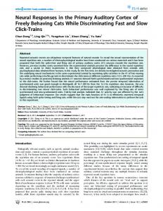
Experimentswere conductedin a double-walledsound-shielded room (IAC). Auditory stimuli were presentedvia calibratedheadphones(STAX 54) enclosedin small chambersthat were connectedto sounddelivery tubessealedinto the acousticmeati (So5 10 kolich 1981; US Patent4251686). The sounddelivery systemwas Frequency @Hz) calibratedwith a soundlevel meter (Brtiel & Kjaer 2209) and a waveform analyzer (General Radio 1521-B). The frequency responseof the systemwasessentiallyflat at zz14 kHz and did not have major resonances deviating more than ?6 dB from the average level. Above 14 kHz, the output rolled off at a rate of 10 dB/octave. Harmonic distortion was ~55 dB below the primary (dependingon the samplingrate and the settingsof the antialiasing low-passfilter.) Toneswere generatedby a microprocessor(TMS32010; 16-bit D-A converter at 120 kHz; low-passfilter of 96 dB/octave at 15, 35, or 50 kHz). Attenuation was provided by a pair of passive 0 0 20 40 60 'f attenuators(Hewlett Packard 350D). The duration of each tone Level (dB SPL) burst was usually 50 ms, except when it was extendedto 85 ms FIG. 2. One-presentation frequency response area (FRA) (A) and correfor long-latencyresponses. The rise-fall time was3 ms.The intersponding spike count-vs.-level function (B) for a nonmonotonic neuron. stimulusinterval was 400- 1,000ms. ,,

I

Gap in dotted background in (A) : l/4-octave band over which spikes were counted. Two spikes on the low-frequency side at 55 dB were outside of Recording procedure the l/4-octave band and thus were not counted for the spike count-vs.level plot. The maximum of 0.8 spikes per repetition seems low because Parylene-coatedtungsten microelectrodes(Microprobe) with the cell was more narrowly tuned than the l/4-octave analysis bin used impedancesof 1.0-8.5 MQ at 1 kHz were introduced into the (see Fig. 12 for more discussion of this methodological effect). The monoauditory cortex with a hydraulic microdrive (KOPF) remotely con- tonicity ratio is calculated by dividing the response at the highest tested intensity, 72 dB, by the largest response. The spike count-vs.-level plot trolled by a steppingmotor. All penetrationswere roughly orthogonal to the brain surface.The recordingsreportedherewere derived incorporates data from another l-repetition FRA (not shown) from the at intracorticaldepthsrangingfrom 600 to 1,000pm, asdetermined same cell that covered from 2 to 72 dB SPL. Also notice that the frequency by the microdrive setting. Dimpling was usually < 100 pm, and range in this example is high resolution (90 frequencies).

thus not a major problem. In severalanimals,histology indicated that recordingswere from layers 3 and 4. Neuronal activity of singleunits or smallgroupsof neurons(2-6 neurons)was amplified, band-passfiltered, and monitoredon an oscilloscopeand an audio monitor. Multiple-unit recordingswere employed only to map the sharpness of frequency and amplitudetuning acrossAI. Recording multiple units allowed for collection of enough data to premaplo-30 cortical locationsin reasonableamountof time (~8 h). Spike activity was isolatedfrom the backgroundnoisewith a window discriminator (BAK DIS-1). The number of spikesper presentationand the arrival time of the first spikeafter the onset of the stimuluswere recordedand stored(DEC 11/73). The recording window had a duration of 50-85 ms,correspondingto the stimulusdurationand excluding any offset response. Data analysis From the responsesto 675 different frequency-level combinations, an objectively determinedfrequency responsearea (FRA) (Fig. 2A) was constructedfor every recording site (for more detailed explanation of FRA procedure see Sutter and Schreiner 1991a). If the resultingFRA was not well defined (subjectively determinedas no responsesfor half of the points in the tuning curve, or for the level of activity encounteredin AI, roughly the standarddeviationof responses greaterthan the mean), the process wasrepeatedwith the same675 stimuli and the resulting evoked activity was addedto the first. The processwasrepeated~5 times until a well-definedFRA wasobtained.This methodhasprovided statistically reliable characterizationof cells basedon repeated-

(Table 3 in Sutter and Schreiner 1991a). Responsemeasures,including peak firing rate, were calculatedfor each stimuluscondition of the FRA by weightedaveragingwith the eight frequency-intensity neighborsas describedpreviously ( Sutter and Schreiner1991a). Spike count-versus-levelfunctionswere derivedfrom eachFRA (Fig. 2B). The functionswere reconstructedby addingaction potentialsfrom a l/4-octave bin centeredaroundthe unit’s CF (usually 4 different frequencies)over 15 dB (3 levels). This provided 2 12 different stimuli for eachtestedintensity per repetition of the FRA procedure.Only units that were testedover a 24%dB range above minimumthresholdwere consideredfor analysisof monotonicity. From the objectively determinedsingle-toneFRAs and spikecount-versus-levelfunctionsseveralresponse propertieswere measured. 1) CF = the stimulusfrequency with the lowest soundpressure level necessaryto evoke neuronalactivity. 2) Minimum threshold= lowestintensity associated with stimulus evoked activity in the FRA. the bandwidth(in octaves)of pure tonesto which 3) Bw4OdB = a cell responds40 dB above minimum threshold(as measured from the frequency tuning curve). For multipeakedunitsthe entire bandwidthencompassing the excitatory response (total bandwidth) was measured. 4) BWlo = the bandwidth (in octaves) of pure tonesto which a cell responds10 dB above minimum threshold(as measured from the frequency tuning curve). For multipeakedunitsthe entire bandwidthencompassing the excitatory response (total bandwidth) was measured.

measures controls

SINGLE-UNIT

INTENSITY

A ‘@Monotonic@ ratio = 0.04

1 4 OO

20

40

60

80

1

l(

Monotonicity ratio = 0.72 A

\

I

40

60

80

193

IN CAT AI

1992). The two nonmonotonic regions can be visualized as two minima in a plot of monotonicity ratio versus dorsoventral location (Fig. 4). To pool data across animals, the two minima in the monotonicity ratio-versus-dorsoventral location plot for each animal were used as normalization points. The monotonicity ratios for all recorded multiple-unit clusters for case SUTCI6 are shown in Fig. 4A. Initially, the most dorsal recording site was arbitrarily assigned a value of 0 (Fig. 4, A and B) . The two highly nonmonotonic regions were - 1.0 and 3.8 mm from the most dorsal recording site. The data were then replotted using a weighted 0.50~mm smoothing algorithm (Fig. 4B, legend). (The convention of placing dashed lines at the 2 minima of the monotonicity ratio used in Fig. 4B is also used in other figures.) From the resulting smoothed curve, the positions of the minima in monotonicity ratio were extrapolated (e.g., Figs. 4B and 5, A and C). Because the ventral and dorsal nonmonotonic regions do not have a spatially exact relationship across animals, distance needed

1

Monotonicity ratio = 1.OO

Monotonic@ ratio = 0.98

40

20

TOPOGRAPHY

A Multiple Units I”-‘-‘-‘-‘-‘-‘-‘-‘000

0

0 0

30

0

OO

000 OO

00 0

0

0 0

20 10 I-/OO

Intensity (dB SPL)

20

40

60

FIG. 3. Spike count-vs.-level functions for 6 neurons. All spikes from an FRA are counted over 15 dB (3 levels, shown by connecting the 3 intensities used for each point) and l/4 octave (5 frequencies). Some are based on > 1 repetition of the FRA procedure and/or were excited by a frequency range of < l/4 octave. The monotonicity ratio is calculated by dividing the response at the highest tested intensity by the largest response.

5) Best amplitude = the stimulus intensity that elicited the most spikes to any tone. 6) Maximum firing rate = the number of spikes, per individual stimulus presentation at the best amplitude. 7) Monotonicity ratio = the number of spikes elicited at the highest intensity level tested divided by the number of spikes elicited at the best amplitude. Single neurons or multiple-unit recordings were classified as monotonic if their monotonicity ratio was >0.8 (Fig. 3C). Units with ratios between 0.50 and 0.80 were classified as intermediately nonmonotonic (Fig. 3B). Monotonicity ratios 50.5 were considered strongly nonmonotonic (Fig. 3A).

Topographic

classijcation

0 1.0 2.0 3.0 410 5 1 Dorsal Cortical Location (mm) Ver ral

80

Intensity (dB SPL)

of single neurons

Because of the difficulty involved in recording enough parametrically fully characterized single neurons to construct a map for each animal, we employed methods for pooling data across animals. Cytoarchitecture, vasculature, and sulcal patterns have historically not been reliable landmarks for pooling (Merzenich et al. 1975)) so we used physiological landmarks to directly compare multiple- and single-unit topography of monotonicity ratio. The pooling method used therefore depends on the multiple-unit intensity-tuning topography, which in this study was consistent with those of Schreiner et al. (1992). The axis for the gradients of sharpness of intensity tuning runs roughly in the dorsoventral dimension, orthogonal to the isofrequency axis (Fig. 1). Two regions of sharp intensity tuning (nonmonotonic regions) consistently can be found along the dorsoventral axis using the multiple-unit technique (Schreiner et al.

B Multiple

a :f 88

Units with Spatial Smoothing

0.8

8 c 0.7 0 1.0 2.0 3.0 410 5-O Ventral Dorsal Cortical Location (mm)

0 -1 z d 0.9 .Q

l’

0.8 d 2 0.7 -1 Dorsal

0

1

2

3

4 Ventral

FIG. 4. Spatial distribution of monotonicity ratio within isofrequency domain (7-9 kHz) for cut SUTCl2. A : multiple-unit data points. B : result of a weighting average spatial smoothing algorithm on the data points. Clusters with the same dorsoventral coordinate were assigned weights of 1.0. Recording sites within 0.10 mm of each other were assigned weights of 0.75. Multiple units between 0.11 and 0.25 mm were assigned weights of 0.5, and neighbors between 0.26 and 0.50 mm were assigned weights of 0.25. The weighted average was calculated to give a “smoothed” value for each data point. The 2 minima in the function are identified by dotted lines. The distance between the minima then was normalized to “3 mrn” (C) , which in this case expanded the real distances by 7%. Notice that in B the map is 5 mm. For all graphs the ventral nonmonotonic region is assigned the value “3” and the dorsal nonmonotonic region is assigned the value “0”.

M. L. SUTTER AND C. E. SCHREINER SUW16

unnormalized

I3 Smoothed Multiple Unit Map 0 Multiple Units +Single Neurons

0.2

I I I I

0.0 I

I

0.4

D

UMOI-IIdiZCd

1.0

+

++I

’

l

5

Cortcal Location (mm)

6

7

8 Ventral

o.oa

-

-1

I I

0

I I I

0.2 ’

! * IO

*

I I

0.4 ’

4

,

0

b I

0.6 9

3

I

SUTc12 normalized I

2

+

l.Oa - -I -v- v - - i 0.8

0 1 Dorsal

I

+ I++ I m I LI

I+

0

lz/i 0.8 p4 2~0.6 ‘d g 04 . 5 g 0.2 E 0.0

+ +++ + 1+

-1 0 1 2 3 4 5 Dorsal Ventral Location Relative Mono Map (mm)

0 1 2 3 4 5 Dorsal Ventral Co&al Location (mm) sml2

SUTC 16 normalized

I 0.8 II I+ 0.6 I

SU’IC 16 OSingleNeurons sUTc12

C

.

1lO

l

!

.

0

1

m 1 0 I ! - .

.

2

3

4

Dorsal Location Relative to Monotonicity

5

6

7

Ventral Map (mm)

E Pooled From SUTC16 and SUTC 12 1.01 - : -+ G -ti ; -r-p

3Q 0.4 ’ g 0.2 ’ b& 0.04#

-

I I I I 4 !

+

++I

+

0

I++ P *

L c 0

I -

1

_

.a!

-

I

:

-

.

-

_

’

-1 0 1 2 3 4 5 6 7 Dorsal Ventral Location Relative to Monotonicity Map (mm) FIG. 5. Illustrative example of pooling method using the 2 cases shown in Fig. 4. The multiple-unit maps ( l - l ) with each single unit (plus signs, cat SUTCl6; open diamonds, case SUTC12) and multiple unit ( 0) are shown for 2 cases (A and C) . Single-unit points (same symbols as in A and C) are displayed after normalization of locations to “3 normalized millimeters” from the multiple-unit map (B and 0). Single units from the 2 cats are superimposed with their common normalized coordinate system (E) . Notice that the point in secondary auditory cortex ( AII) ( C and 0) is not included in final pooled data.

to be normalizedto usethesetwo locationsaspooling landmarks. The distancebetweenthe two minimarangedbetween2.8 and 3.4 mm, with a meanof 3.1 (median3.05, N = 5)) and thereforewas normalizedto “3.0” mm (transformationfrom Fig. 4, B to C) , approximatingthe medianvalue of 3.05. For the casedepictedin Fig. 4, normalizationdistorted distanceby -7%. This distortion canbe seenby directly comparingFig. 4, B and C. In real distance the penetrationsfrom this animalcover slightly G.0 mm in dorsoventral extent (Fig. 4B) ; however, after normalizationthe penetrations occupy >5 mm along the distorted normalized axis (Fig. 4C). After normalization,the dorsalandventral monotonicityratio minima were arbitrarily assignedlocations of 0.0 and 3.0 mm, respectively. The methodof pooling data acrossanimalsis illustratedin Fig. 5. The unnormalizedspatial distributions of single neuronsare shownsuperimposed on the smoothedmultiple-unit maps(0) for two cats in Fig. 5, A and C (A, cat SUTCl6; C, cat SUTC12). The multiple-unit mapsare normalized as previously described, and the locations of single neuronsare assignedabscissavalues

from the normalized coordinatesystem(Fig. 5B, SUTCl6; Fig. 5 D, SUTCl2). For case SUTCM (Fig. 5, A and C), singleneurons’ monotonicity ratios are representedby plus signsand for case SUTCl2 (Fig. 5, B andD) they arerepresented by diamonds. After normalization,singleunitsfor both caseshavebeenassigned valuesrelative to the monotonicitymapandaredirectly comparable (compareplus signsand diamondsin Fig. 5E with thoseof Fig. 5, B and D). The samepooling process,as demonstratedin Fig. 5 for cats SUTCl2 and SUTCM, was repeatedfor all other cases. To enablecomparisonsof intensity-dependentpropertieswith previous studies,we alsousedthe integratedexcitatory bandwidth of multiple-unit recordings ( Schreiner and Mendelson 1990; Schreinerand Sutter 1992) as a pooling landmark. For pooling relative to bandwidth, we usedthree measures:the dorsoventral locationwherethe multiple-unitresponses have the sharpesttuning 40 dB above threshold( BWdoen) , the dorsoventrallocationwhere the multiple-unit responses have the sharpesttuning 10 dB above threshold ( BWlo min),and a compositeof the two (BW10,40 min), namely the averagelocation of the BWI0 tin and BWa fin.

SINGLE-UNIT

INTENSITY

TOPOGRAPHY

A

RESULTS

Results are based on recordings of 108 single neurons recorded from nine cats. Single-neuron recordings were topographically localized with respect to known multiple-unit maps. Single-neuron population results were compared with 147 multiple units that were recorded in the initial mapping procedure from the same set of experiments. We found neurons with a wide range of monotonicity ratios (Fig. 3). Throughout AI, single-neuron recordings yielded a higher percentage of nonmonotonic responsesthan did multiple-unit recordings. Single neurons, particularly those in AIv, tended to have a steeper reduction of activity at high intensity levels (i.e., smaller monotonicity ratios) than was observed for multiple-unit responses.Although the multiple-unit topography had two clear nonmonotonic regions, the dorsal nonmonotonic region was difficult to reconstruct from single-unit data. Furthermore, we saw more local topographic scatter in monotonicity ratio and minimum threshold for single neurons than for multiple units. Differences between single- and multiple-unit monotonicity ratio topographies can be accounted for by two separate results. I) There was a greater scatter in intensity thresholds in monotonic regions. The nonmonotonic regions, with lower threshold scatter, contain neurons with similar best amplitudes. 2) Nonmonotonic neurons contribute more spikes in topographically nonmonotonic regions than in topographically monotonic regions.

li

n=

IN CAT AI

10

19

195

17

23 22 10 17 5

EO. -3 0

-.corsal Locltion B

n=

4

11

I I

Relative t”oMonotonici;

10

+

+I +I

+ +

+

I

0.01

Pooled monotonicity

data

For multiple-unit recordings,pooling did not distort the topographic distribution of monotonicity ratio, which had a similar shape to that described for individual cases.We observed a weak nonmonotonic region near the dorsalnonmonotonic referenceand a stronger nonrnonotonic region -3 mm ventral (Fig. 6A). A third nonmonotonic region can be seenat the ventral

c 1.o ---B111 Mu1tip1e Unit

2 . $$ l

Jj 0.7% -

zi g OA&! . nc 1 V.J

+ I

c

-2 -1 0 1 2 3 4 5 6 Ventral Dorsal Location Relative to Monotonic@ Map (mm)

topography

As reported in an earlier paper ( Schreiner et al. 1992), we observed a dorsal and a ventral nonmonotonic region in AI. In some cases(4 of 9) we found a gradient with increasing sharpnessof frequency tuning toward the ventral extreme of AI. In these animals it appeared that this gradient was leading to a third nonmonotonic region in or near the secondary auditory cortex (AII). Although the intensity-dependentresponseproperties of single neuronsand multiple units were different in somerespects, the locations of the major minima and maxima of the monotonicity ratios of single- and multiple-unit responsescorresponded. Single neurons,on average, had lower monotonic&y ratios and much wider rangesof monotonicity ratios at a given dorsoventral location than did multiple units (e.g., Fig. 5). The singleneuron topography was qualitatively similar to the multipleunit topography for the two animalswith the largest single-unit samples,SUTCl2 and SUE16 (Fig. 5). Although similarities between single and multiple units can be seen,the significance is hard to determine becauseof the large scatter in values for a given dorsoventral location, the small number of samples, and the sharpertuning of single units. Therefore pooling data across animals was necessaryfor quantitatively verifying the observed single-neuroncontributions.

” Ventral

Map (mm)

18 14 13 13 11 7

4

monotonic@

5

1.0

I

Within-experiment

14

.

-

Single Unit

I

\ i

r’

4 5 6 -2 -1 0 1 2 3 Dorsal Location Relative to Monotonicity Map (mm)Ventral

FIG. 6. Scattergram of pooled monotonicity ratio data for (A ) multiple units and (B) single units. A : dashed line connecting filled rectangles displays the mean monotonicity ratios of multiple units averaged over OS- or 1.0~mm bins; rectangles are located at the center of the bins. Bins of 0.5 mm were used if 2 10 neurons were located within the bin; otherwise 1.Omm bins were used. The numbers of recordings in each bin are displayed at the top of each graph. B: similar curve for single neurons. C: mean binned results for single and multiple units with magnified monotonicity ratio scale. For all plots, vertical dashed lines represent the normalization points used, i.e., center of the dorsal and ventral nonmonotonic regions as determined by multiple-unit mapping.

extreme of AI (from 5 to 6 mm) for both multiple- and singleunit topographies.This is causedby the occasionally encountered nonmonotonic region near the AI-AH border. For the pooled data, differences in the details of multiple-

196

M. L. SUTTER AND C. E. SCHREINER

and single-unit responseproperties can be seen throughout the dorsoventral extent of AI, but in AIv the general structures of multiple- and single-unit topographies were similar. Single units responded with a wider range of monotonicity ratios than multiple units throughout the entire dorsoventral extent of AI (Fig. 6, A and B). Single units also on average were more sharply tuned for intensity than multiple units. Although the wider variability and sharper intensity tuning of single units is apparent, in AIv there is a correspondence of the topographic gradients (Fig. 6C). A minimum in monotonicity ratio is located in the ventral nonmonotonic region as determined by multiple-unit mapping. This minimum is accompanied by an ascending gradient in monotonicity ratio for - 1.5 mm in either direction for both multiple and single units. In AId, however, there is no correspondence of the pooled topographies. The multiple-unit gradient of monotonicity ratio starts descending from a maximum at -2 mm from the dorsal nonmonotonic region, then reaches a minimum at the center of the dorsal nonmonotonic region and reverses (Fig. 6, A and C). The topography of singleunit monotonicity ratio, however, is relatively flat, except at the dorsal extreme, which only has a sample of four cells (Fig. 6B). The difference between single and multiple units in AId indicates that local differences in single-unit scatter or the spike contribution of sampledcells are generating the observed multiple-unit gradients. The topographic variation of correspondence between single- and multiple-unit responsesdemonstrates that there are physiological and/or organizational differences between dorsal and ventral nonmonotonic regions. One might ask whether regions of low monotonicity ratio are a result of a few strongly nonmonotonic cells or of many intermediately nonmonotonic cells. From Fig. 6, A and B, it appearsthat AId has fewer strongly nonmonotonic neurons than AIv, but a similar proportion of intermediately nonmonotonic cells. However, it is difficult to determine percentagesfrom this figure becausethere are many cells with a monotonicity ratio of 1 with overlapping symbols. To address this question quantitatively, we classified neurons as monotonic (monotonicity ratio > 0.8)‘) strongly nonmonotonic (monotonicity ratio < 0.5), or intermediately nonmonotonic (monotonicity ratio between 0.5 and 0.8). A criterion of 0.8 as the monotonic-nonmonotonic cutoff is somewhat arbitrary and was chosen to be conservative in classifying a unit as ‘ ‘monotonic. ’ ’ The percentage of nonmonotonic multiple units plotted versus pooled location shows the spatial distribution that would be expected from the monotonicity ratio topography (Fig. 7A). Namely, locations with >50% nonmonotonic neurons are aligned with the locations that have the lowest monotonicity ratios. There were, however, only a few strongly nonmonotonic multiple units. No spatial bin contained >25% of strongly nonmonotonic multiple units. The small number of strongly nonmonotonic multiple-unit responsesroughly inversely followed the spatial distribution of monotonicity ratio. The percentage of intermediately nonmonotonic multiple-unit responses shows a more pronounced spatial distribution very similar to the expectations from the maps shown in Fig. 6C. These results indicate that the spatial distribution of multiple-unit monotonicity ratio is a result of an increase in the percentage of nonmonotonic multiple-unit responsesat certain locations.

n

Strongly Non-monotonic

m

(% Reduction c 50)

Intermediately Non-monotonic

(% Reduction Between 51 and 80)

A n= 10 80

19 17

23

22

I

10

17

5

14

5

I

1

60

40

,

20

0 il.5 -0.5 0.5 1.5 2.5 3.0 3.5 4.0 4.5 5.5 6.5 Dorsal Ventral Location Relative to Monotonic&y Map (mm) B n=

-

4

11

10 18

14

13

13

11

7

0.5 1.5 2.5 3.0 3.5 4.0 4.5 5.5 Dorsal Ventral Location Relative to Monotonicity Map (mm)

RG . 7. Percentage of strongly nonmonotonic (filled) and intermediately nonmonotonic ( hatched) neurons for topographically pooled multiple (A ) and single (B) units. Number of units pooled for each bin is shown by y1 value at top of each plot.

For single neurons, a similar straightforward explanation of the spatial distribution of monotonicity did not apply to all cortical locations. Although the distribution of the percentage of nonmonotonic single neurons followed the topographic distribution for monotonicity ratio in AIv, this was not as clearly expressed for the dorsal third of AI (Figs. 6C and 7B). Although the percentage of nonmonotonic neurons in AId was similar to that in the central and ventral regions ( >60%), there was a lack of strongly nonmonotonic neurons ( < 10%) in AId. The high percentage of intermediately nonmonotonic neurons in AId is another property that physiologically distinguishes it from AIv. The differences in the sharpnessof intensity tuning between neurons of dorsal and ventral nonmonotonic regions contribute to the apparent

SINGLE-UNIT

3 3

INTENSITY

I

I

g * z g0 2EI g * z ‘S O l2 2 * ld 3 0

I

-

I.1

-,

-

I.

I.

I

-

-1.5 -0.5 0.5 1.5 2.5 3.5 4.5 5.5 6.5 Ventral Dorsal Location Relative to Mono Map FIG. 8. Ratio of spikes contributed from nonmonotonic units and monotonic units. Maximum spike count per stimulus to tones (FR,,,) was calculated for each neuron. Within each bin, FR,,, was added for all nonmonotonic neurons, and this sum was then divided by the equivalent measure for monotonic neurons. Notice that a maximum of the ratio occurs both in the dorsal and ventral nonmonotonic regions.

topographic differences between single-and multiple-unit maps. Contribution of firing rate and threshold There are at least two additional factors contributing to how a multiple-unit monotonicity topography can be created in AId, whereas a similar topography is less evident in the monotonicity of single neurons. One is that nonmonotonic neurons contribute more spikes to cluster responsesin nonmonotonic regions than do monotonic neurons. The other is that thresholds of neurons might be similar in nonmonotonic regions. The resulting frequency tuning curves of nonmonotonic single neurons in nonmonotonic regions thus would be superimposed on each other, creating a multiple-unit responsethat is tuned for intensity. By contrast, when looking at multiple-unit responses,the threshold scatter in the monotonic regions would obscure the intensity tuning of individual neurons. Part of the difference between multiple and single units in AId is due to nonmonotonic neurons contributing more spikes than monotonic cells. For every neuron we calculated the firing rate at the best amplitude (FR,,,). Within each OS- or l.O-mm bin, this firing rate was added for all nonmonotonic single neurons (FRmaxnonmono). FR,, was also added for all monotonic neurons in each bin to arrive at FRmax mono to max mono was then divided by FRmaxnonmono arrive at the spike ratio for any given location (Fig. 8). Ratios > 1 indicate that nonmonotonic neurons, on average, contributed more spikes at best intensity than monotonic neurons. The spatial distribution of spike ratios parallels that of multiple-unit monotonicity ratios in the dorsal nonmonotonic region. Notice that between 0.0 and 2.0 mm the spatial distribution of single-unit spike ratio is different than that of the single-unit monotonicity ratio (Fig. 6). The singleunit spike ratio shows a gradient consistent with the multipleunit topography of monotonicity ratio (Figs. 6 and 8), whereas the single-unit monotonicity ratio map is flat. Differential contribution of spikes between monotonic and nonmonotonic neurons, therefore, at least partially contribute to the formation of a multiple-unit topographic representation

TOPOGRAPHY

IN CAT

197

AI

of monotonicity from a relatively nontopographic singleneuron distribution in AId. Changesin threshold scatter also contribute to the creation of ‘ ‘monotonic regions’ ’ from underlying nonmonotonic cells. Single-neuron thresholds were less scattered in the multiple-unit nonmonotonic regions than they were in the mapped monotonic regions. This was apparent in individual casesas well as in the pooled data (Fig. 9). Notice that in the nonmonotonic region near the AI-AI1 border the scatter was large, probably reflecting the increased neuron thresholds observed as the AI-AI1 border is approached (Schreiner and Cynader 1984). Thresholds in the dorsal and ventral nonmonotonic regions of AI were among the lowest thresholds recorded in each animal (Fig. 9B). The superpositionof responsesfrom nonmonotonic neurons with low thresholds contributes to the creation of regions of nonmonotonic multiple-unit responses. Relation of monotonicity topography to BW topography The monotonicity topography is related to the sharpness of frequency tuning topography reported in previous studies (Schreiner and Mendelson 1990; Schreiner and Sutter 1992;

Alog

0 Monotonic 0 Unclassifiable Monotonicity a Strongly non-Monotonic + Intermediate Non-monotonic - * - -

t

0

8i 0

0 l

+

0

0

+

+ 0

0

301

0

0

0

0

X 000

X

c, 4,

/

1

1

2

3

4

5

1

2

3

4

5

6

w

FR

l

-2 Dorsal

-1

0

Location Relative to Monotonicity Map (mm)

6

Ventral

FIG. 9. Threshold data pooled across animals. Zero and 3 mm correspond to 2 nonmonotonic regions. The line drawn at 3 mm for all other figures has been omitted to allow for better viewing of the data. Threshold was referenced such that for each animal 0 dB corresponded to the lowest multiple-unit threshold encountered. Notice the minima in threshold scatter at the 2 nonmonotonic regions and the threshold minimum at the ventral nonmonotonic region. Unclassifiable Monotonicity (A, O) refers to cells in which monotonicity ratio could not be calculated because 45 dB SPL; however, at intensities >45 dB there were still responses at frequencies below the CF. The low-frequency response causes the FRA-determined spike countversus-level profile to fall off less steeply than the PSTHdetermined spike-versus-level profile ( Fig. 12A ) . Nonmonotonic neurons with oblique or tilted frequency tuning curves have been previously shown (e.g., Fig. 3 in Phillips et al. 1985). Many of the intermediate nonmonotonic neurons identified in this study had oblique frequency tuning curves. There is no evidence that the intermediate nonmonotonic neurons, as defined in this study, had spike-versus-level functions asymptoting at intermediate response rates. In-

stead, almost all intermediate nonmonotonic neurons showed a downward slope of their spike-versus-level functions at the highest tested intensities (e.g., Fig. 3). Becausethe intermediately nonmonotonic neurons had not reached an asymptote or zero response at the highest intensity tested, we can neither confirm nor rule out the existence of nonmonotonic neurons that asymptote at intermediate intensities. Another methodological consideration is the recording depths encountered in this study. Although histology has confirmed that recordings were restricted to layers 3 and 4 in several animals, we cannot rule out the possibility that some recordings extended beyond these boundaries in animals for which no histology was performed. This should not pose a problem because the number of such recordings would have to be minimal and thus would be averaged out by pooling. This study did not investigate the effects of depth

200

M. L. SUTTER AND C. E. SCHREINER

A2

A -+-

?-A I 9 \ I \ \ : O- O\ I

PSTH 50 Reps FRA 0.1 octave width FRA 0.25 octave width

80 Intensity (dB SPL) - -O- - FRA 0.1 octave width PSTH first 5 reps

20

40

60

80

Intensity (dB SPL) FIG. 12. Habituation effects of the peristimulus time histogram (PSTH) method for neuron whose FRA is depicted in Fig. 2. A: comparison of spike count-vs.-level plot derived from 50-repetition CF tone PSTHs with measures derived from FRAs. Notice that the 0.25-octave window used underestimates spikes per presentation. This is because the neuron’s frequency tuning curve (FTC) is 20 dB) is less sharply sloped for the FRA method compared with PSTHs. This is because at high intensities, to which the CF response is substantially reduced, off-CF responses are still present (see Fig. 2).

on single-unit topography, but rather attempted to sample from a slab corresponding to layers 3 and 4. While multipleunit maps of intensity are stable with recording depth (Schreiner et al. 1992), single-unit topographies need not be. Therefore the effect of recording depth is still an open question. Interanimal variability Recent multiple-unit mapping studies (Heil et al. 1992b; Schreiner et al. 1992) have reported reproducible topographic distributions of bandwidth and intensity in cat AI. Although, general features of the topography are highly reproducible, there is a high degree of interanimal variability

in the details of the topographies. The details of interanimal variability are lost in the pooling process.Pooling data across animals, however, allows us to compare the most reliable and reproducible aspectsof the topographies acrossanimals for single and multiple units. In these studies, the reliable topographic landmarks are a region of multiple-unit responsessharply tuned for frequency and two regions of multiple-unit responsessharply tuned for intensity (Heil et al. 1992b; Schreiner and Mendelson 1990; Schreiner et al. 1992). Our ability to obtain pooled results on the basis of these topographic properties is a testament to the reliability of these aspectsof the multiple-unit topography from animal to animal. Our method, however, ignores the interanimal variability described in these topographies. Therefore it is important to remember that the goal of these experiments was to compare multiple- and single-unit responses.In single-unit studies, one cannot obtain a large enough extent and fine enough resolution to measure idiosyncratic interanimal variability over completely mapped areas (which requires 961 locations to map out a 6 X 6 mm grid with 200~pm resolution). Additionally, pooling single- and multiple-unit data within the same animal will yield irregular maps because of differences in single-unit and multiple-unit topographies (Schreiner and Sutter 1992). Comparing singleunit and multiple-unit topographies allows us to gain a better understanding of the basic features of single-unit topography underlying the observed multiple-unit properties. An argument can be put forth that our not finding a pooled monotonicity ratio gradient for single units in AId is due to interanimal variability. It is possible that within each animal there is a weak single-unit gradient for monotonicity ratio. However, there are several arguments against pooling being the sole reason for the absenceof a gradient of pooled singleunit monotonicity ratio in AId. First, we do see a gradient for pooled multiple-unit mapsof intensity parametersin AId. Therefore, if interanimal variability is the cause of the lack of a gradient, the variability has to be constrained to single units while not being present in multiple units. Second, we see spatial gradients of spike ratio and threshold for single units in AId. These results indicate that the lack of spatial gradient or very weak spatial gradient of monotonicity ratio in AId is not solely a result of pooling data acrossanimals. Comparison with previous studies The percentage of nonmonotonic neurons reported in this paper is consistent with previous results in cat AI. Recent studies from the cat have reported that approximately half of AI cells are nonmonotonic. When comparing neuron populations across investigators, the possibility of topographic sampling biases (particularly toward central and ventral AI in recent reports) must be kept‘in mind (Sutter and Schreiner 199la). Recording from similar cortical depths, Phillips et al. ( 1985) found that 44% of single neurons (A7 = 61) are strongly nonmonotonic, 13% intermediately nonmonotonic, and 43% monotonic. In a preliminary disclosure, Barone and colleagues ( 1990) have reported that 40% (data baseof 333 neurons) of recorded AI neurons were strongly nonmonotonic. In all regions of AI, the reported percentage of nonmonotonic neurons in this paper is similar to those of previous studies. In the 2 mm of the dorsoventral extent of AI centered on B W10j40tin, 33% of neurons are strongly non-

SINGLE-UNIT

INTENSITY

monotonic, 28% are intermediately nonmonotonic, and 39% are monotonic. Dorsal to this region 10% are strongly nonmonotonic and 38% are intermediately nonmonotonic. Ventral to this region, 35% are strongly nonmonotonic and 19% are intermediately nonmonotonic. These results are consistent with previous findings that roughly 40-60% of AI neurons are nonmonotonic (see also Figs. 7 and 11). The results from the central and ventral region are consistent with the findings that most nonmonotonic neurons in “classical” AI are strongly nonmonotonic (Phillips et al. 1985). The percentage of nonmonotonic neurons is substantially different between AI of the cat and AI of the mustached bat. Most of the neurons in bat AI are intensity selective, although only 25 of 153 ( 16%) were completely inhibited at high intensities (Suga and Manabe 1982). Of 540 neurons in the same study, only 19 were monotonic. If we assume then that at most 19 of 153 neurons were monotonic, then ~87% of bat AI neurons were nonmonotonic and ~71% of AI neurons were intermediately nonmonotonic. The results of Suga and Manabe indicate that the percentages and strengths of nonmonotonic neurons in AI can vary substantially across species. This interpretation, though, is subject to a severe limitation because of differences between free-field and dichotic stimulus presentation methods. In the bat study auditory stimuli are presented free field, whereas in the cat stimuli were presented monaurally. The percentages of nonmonotonic units found in the medial geniculate body (MGB ) and inferior colliculus (IC) indicate that higher percentages of nonmonotonic neurons are reported in experiments performed under free-field conditions. In free-field studies of the cat, 80% ( Aitkin 1991) of IC neurons were nonmonotonic. However, recording from MGB under monaural conditions there is a progression in the percentage of nonmonotonic neurons from 30% in the anterior portion to 60% in the posterior portion of MGB of the cat (Rodrigues-Dagaeff et al. 1989). Under monaural stimulation conditions in the guinea pig, 24% of IC neurons were nonmonotonic (Rees and Palmer 1988). Across these experiments neuronal recordings performed under free-field conditions consistently result in a larger percentage of nonmonotonic cells than dichotic contralateral stimulation. One might expect to see higher percentages of nonmonotonic neurons under free-field conditions because of neurons suppressed by the ipsilateral ear with higher thresholds than the excitation threshold in the contralateral ear. Confounding the results further are the different manners in which investigators define the boundaries of brain regions. The relatively few studies of amplitude processing in the CNS, coupled with a large variation in methodologies used, make it difficult to conclude whether there are species-dependent or brain-region-dependent differences in the percentages of nonmonotonic neurons. Although the percentage of nonmonotonic neurons may be different between cat and mustached bat, topographic representations of stimulus intensity can be observed in both species. Besides the cat, functional maps of amplitude related parameters in AI only have been demonstrated in bats. In the mustached bat there is a map of best amplitude that runs roughly orthogonal to the frequency map ( Suga 1977; Suga and Manabe 1982). For echolocation, the amplitude of the returned pulse conveys information about object size. The findings of topography of monotonicity and best level in the

TOPOGRAPHY

IN CAT

AI

201

cat (Schreiner et al. 1992) combined with the single-neuron results presented in this study indicate that a topographic representation of intensity parameters might be a general mammalian auditory cortical property. For both species, the amplitude of the stimulus also appears to be encoded orthogonal to the tonotopic axis in AI. Although Suga and Manabe did not study the sharpness of amplitude tuning (they studied best level), there is some indication that there is an orderly organization of degree of monotonicity (see Fig. 10 in Suga and Manabe 1982). Possible mechanisms

creating nonmonotonicity

An argument can be put forth that neuronal intensity tuning is solely a result of the broader-frequency response of the basilar membrane at higher intensities (von Bekesy 1960; Rhode 197 1; Ruggero and Rich 199 1) impinging on inhibitory sidebands. The broadening of tuning is due to the mechanical properties of the basilar membrane and effects of stimulus shaping. Therefore under these circumstances lateral inhibition is converted to intensity tuning. If a splattering of energy into inhibitory sidebands is contributing to the creation of intensity-selective neurons, one would expect to find inhibitory sidebands -40 dB below the highest intensity at which the cell is excited. However, low excitatory thresholds, such as those reported for cells in the nonmonotonic areas, are unrelated to this potential mechanism. Phillips ( 1988) has provided evidence that spectral splatter from inhibitory sidebands contributes to intensity tuning by demonstrating that for some nonmonotonic cells intensity tuning becomes sharper with more rapid tone onsets. On the basis of nonmonotonic cells’ responses to broadband noise, Phillips and Cynader ( 1985) have also hypothesized that nonmonotonicity might arise from inhibitory neurons with similar CFs but higher thresholds. We have recently collected data demonstrating that nonsideband high-threshold CF inhibition contributes to intensity tuning (unpublished observations). These results demonstrate that the auditory system can use sideband (lateral) and/or nonsideband inhibition to create intensity tuning. Although it is probable that sideband inhibition contributes to intensity tuning, this does not argue that intensity tuning observed in AI is not functionally relevant. Establishing the significance of intensity tuning is a behavioral and functional issue, and not only an issue of mechanism. In fact, one would expect the auditory system to exploit spectral splatter for intensity analysis because this is a natural property of sound stimuli. Functional

signiJicance of intensity tuning

Although many studies have been devoted to determining the functional role of the auditory cortical fields, a resolution of distinct functions has not been achieved. There is strong evidence that the AI is involved in sound localization (e.g., Heffner and Master-ton 1975; Jenkins and Merzenich 1984; Thompson and Cortez 1983). There is also data that support the hypothesis that AI is involved in performing vocalization analysis (Coslett et al. 1984; Gazzaniga et al. 1973; Heffner and Heffner 1986a,b, 1989a,b). In bats there is evidence that auditory cortex performs temporal-spectral analysis (Simmons et al. 1990; Suga 1989).

202

M.

L. SUTTER

AND

In addition to sound localization, temporal-spectral analysis, and vocalization analysis, there is a large body of data indicating that auditory cortex is involved in analyzing the intensity of time-varying frequency components composing auditory scenes (e.g., Dear et al. 1993; Simmons et al. 1990). The presence of intensity maps in AI provides strong circumstantial evidence that AI is contributing to intensity analysis (e.g., Suga and Manabe 1982). Although long-duration, pure-tone suprathreshold intensity discrimination seems to be intact in animals with auditory cortical lesions (Neff et al. 1975; Swisher 1967), intensity discrimination appears to be impaired for short-duration tones (Cranford et al. 1982). Additionally data from complex signal discrimination and detection experiments (Blaettner et al. 1989; Heilman et al. 1973; Olsen et al. 1975; Simmons et al. 1990), lesion studies ( Auerbach et al. 1982; Ferrier 1876, 1889; Heffner and Heffner 1986a, 1989a, 1990; Jerger et al. 1969; Muruyama and Kanno 1961) , and sound-localization studies (Imig et al. 1990; Rajan et al. 1990a) provide evidence that the auditory cortex is involved in low-intensity signal detection, amplitude-spectrum analysis, signal-noise analysis, and amplitude modulation analysis. Auditory cortex has been shown to be involved in analyzing many attributes of signals. The physiological organization of auditory cortex is well suited for such multidimensional analysis. In AI of the mustached bat, cells are tuned to Doppler-shifted frequency (Suga and Jen 1976), amplitude spectrum (Suga 1977), echo delays (Fitzpatrick 1993), and specific intraspecies communication vocalizations (Kanwal et al. 1993; Ohlemiller et al. 1993). Like the bat, AI of the cat has representations of multiple signal parameters (Schreiner et al. 1988). The presence of multiple auditory cortical fields and subdivisions of these fields argues for multiple functions in auditory cortex. Therefore it is reasonable to suppose that AI can be involved in processing many different signal parameters. Ultimately the only way to address the functional significance of the intensity maps reported in this paper directly is to perform combined behavioral and physiological studies of the role of AI in intensity analysis. Implications

for sound localization

Recently there has been a resurgence in interest in sound localization sensitivity of AI neurons ( Ahissar et al. 1992; Rajan et al. 1990a,b). Nonmonotonic neurons have been shown to be predominantly directionally selective (Imig et al. 1990). The spatial distribution of minimum thresholds (Fig. 9) indicates that the ventral multiple-unit nonmonotonic region with its restricted intensity response and threshold range cannot encode intensity-independent location. Although the cells in this topographic region would likely be directionally selective, the paucity of monotonic cells that could fire at high intensities indicates that this region can only encode location at low intensities. This, coupled with the fact that monotonic cells are less likely to be directionally selective, makes the ventral nonmonotonic region a poor candidate for level-tolerant spatial encoding. The monotonic multiple-unit regions would be better candidates to serve such a function, because there is a full representation of intensities (including many monaurally nonmonotonic single neurons and possibly more free-field nonmonotonic neu-

C. E. SCHREINER

rons) . The recent data, however, indicate that a simple intensity-tolerant map of auditory space is unlikely to be found within cat AI. Possible purpose detection?

of nonmonotonic

regions: signal

If the nonmonotonic multiple-unit regions in AI are not encoding intensity-independent location information, what are they encoding? One possibility is that the strongly nonmonotonic neurons are encoding spectral information just above the background noise. The ventral nonmonotonic region, which closely overlaps BWdO fin, could serve this purpose well. The hypothesis of an area specialized for signal analysis just above background noise is supported by 1) the low thresholds of these neurons (Fig. 9)) 2) the low scatter in frequency and threshold values, 3) the sharp frequency tuning, 4) the permanent increases in intensity thresholds after AI lesions (Heffner and Heffner 1986a, 1990; Muruyama and Kanno 1961) , and 5) the effect of an increase in background noise on the responses of nonmonotonic neurons (Phillips 1985, 1990; Phillips and Cynader 1985). Neurons in the ventral nonmonotonic region consistently had the lowest thresholds within the isofrequency domain and have the smallest range of threshold values (Fig. 9). This implies that the intensity sensitivity is restricted to a small range of low levels. When tones are presented in the presence of continuous (ongoing) background noise, the spike countversus-intensity function of nonmonotonic neurons shifts as a linear function of the intensity of the noise masker (Phillips 1985, 1990; Phillips and Cynader 1985). Along with the prediction that neurons in the ventral nonmonotonic regions are able to shift their spike count-versuslevel functions relative to background noise, these neurons respond to a narrow range of frequencies and respond weakly if at all to broadband stimuli (Phillips et al. 1985; Schreiner and Mendelson 1990; Schreiner et al. 1988). Accordingly the spectral analysis of signals close to the background signal benefits from a narrowband analysis. Limiting bandwidth enables the neurons to use coherent modulations to detect signals in noise. The ventral nonmonotonic region approximately lines up with BWlo fin, BWdo An, and the lowest threshold region. Topographically, the region near the “physiological center’ ’ of AI is highly selective for detecting the frequency and amplitude of narrowband stimuli just above the background noise, and might be interpreted as a subregion specialized for signal detection. The narrowband frequency response of this area and the spatial selectivity of nonmonotonic neurons (Imig et al. 1990), combined with their low thresholds, indicate that the two nonmonotonic regions may play an important role in spectral-spatial processing for stimuli whose intensities are within -40 dB of the detection threshold of background noise. Note that natural stimuli to which this region would respond must contain at least one narrow band because most nonmonotonic units do not respond well to broadband stimuli (Phillips et al. 1985; Schreiner and Mendelson 1990). Parceling

of AZ

The results of this study raise some questions about the division of AI. Recent papers (Schreiner and Sutter 1992:

SINGLE-UNIT

INTENSITY

Sutter and Schreiner 1991a) have suggested that there are at least two physiologically distinct regions in AI. In AId there is a single-unit map for stimulus bandwidth. Broadly tuned neurons are located dorsally and there is a gradual progression of narrower tuning toward the dorsoventral center of AI. In AIv, most single units are sharply tuned for frequency. The amplitude tuning described in this paper provides further support for the physiological subdivision of AI into two parts. In AIv, where there is no topographic gradient for the bandwidth of single units, there is a single-unit map for stimulus intensity. However, in AId, where there is a single-unit map for bandwidth, there is no single-unit map for stimulus intensity. Although subdividing AI into at least two physiological subdivisions is supported by the data from this and other studies, the dividing line between AIv and AId remains uncertain. The implied dividing line from the previous study was BW10/40 min (Q-max in Sutter and Schreiner 1991a) as derived from multiple-unit mapping of BWdOdB and In this study, BW10,40tin was not as strong a topoBWlOdB* graphic pooling landmark as was BWdOdB or the monotonicity map. The topographic analysis for monotonicity was critically dependent on using high-intensity properties of neurons. With this in mind, the question must be raised as to whether there is a clear dividing line between AId and AIv. The answer appears to be that there is no sharp boundary or unambiguous line that can be drawn to determine functionally distinct AI regions. The AIv-AId classification of Schreiner and Sutter ( 1992) was adequatefor studying bandwidth properties. For studying the spatial distribution of a given filter property, the multiple-unit topography of that property serves as the best topographic pooling landmark. The BWdOdBmap probably is the most useful predictor of the location of other responseproperties studied up to this time. A low-threshold region, with neurons sharply tuned for frequency and amplitude, comprises about 5 1 mm from Ventral to BW40 An, almost all single neurons are BW40min* sharply tuned for frequency, and there is a single-unit map of stimulus intensity. Dorsal to BWdOtin, there is no clear single-unit map of intensity, but there is a gradient for bandwidth. The sharpnessof frequency tuning in AId closely follows the multiple-unit map, whereas amplitude tuning does not. The construction of the dorsal nonmonotonic region, which is present in multiple-unit monotonicity map but not in pooled single-neuron maps, can be accounted for by a combination of threshold scatter and the differential spike contribution of single neurons. This work was supported by Office of Naval Research Grant N0001491-J-1317. Present address of C. E. Schreiner: Center for Neuroscience, University of California Davis, Davis, CA 95616. Address for reprint requests: M. Sutter, University of California, Davis Center for Neuroscience, 1544 Newton Ct., Davis, CA 95616. Received 28 December 1993; accepted in final form 12 September 1994. REFERENCES M., AHISSAR, E., BERGMAN, H., AND VAADIA, E. Encoding of sound-source location and movement: activity of single neurons and interactions between adjacent neurons in the monkey auditory cortex. J. Neurophysiol. 67: 203-215, 1992. AITKIN, L. Rate level functions of neurons in the inferior colliculus of cats AHISSAR,

TOPOGRAPHY

IN CAT AI

203

measured with the use of free-field sound stimuli. J. Neurophyisol. 65: 383-392, 1991. AUEREIACH, S. H., ALLARD, T., NAESER, M., ALEXANDER, M. P., AND ALBERT, M. L. Pure word deafness. Analysis of a case with bilateral lesions and a defect at the prephonemic level. Brain 105: 27 l-300, 1982. BARONE, P., IRONS, W. A., CLAREZY, J. C., AND IMIG, T. J. A comparison of the directional properties of nonmonotonic neurons in the auditory thalamus and primary auditory cortex (AI) of cat. Sot. Neurosci. Abstr. 16: 719, 1990. VON BI?KJ&Y, G. Experiments in Hearing, translated and edited by E. G. Wever. New York: McGraw-Hill, 1960. BLAETTNER, U., SCHERG, M., AND VON CRAMON, D. Diagnosis of unilateral telencephalic hearing disorders. Evaluation of a simple psychoacoustic pattern discrimination test. Brain 112: 177- 195, 1989. BRUGGE, J. F., DUBROVSKY, N. A., AITKIN, L. M., AND ANDERSON, D. J. Sensitivity of single neurons in auditory cortex of cat to binaural tonal stimulation; effects of varying interaural time and intensity. J. Neurophysiol. 32: 1005-1024, 1969. COSLETT, H. B., BRASHEAR, H. R., AND HEILMAN, K. M. Pure word deafness after bilateral primary auditory cortex infarcts. Neurology 34: 347-352, 1984. CRANFORD, J. L., STREAM, R. W., RYE, C. V., AND SLADE, T. L. Detection versus discrimination of brief-duration tones: findings in patients with temporal lobe damage. Arch. Otolaryngol. 108: 350-356, 1982. DEAR, S. P., SIMMONS, J. A., AND FRITZ, J. A possible basis for representation of acoustic scenes in auditory cortex of the big brown bat. Nature Land. 364: 620-623, 1993. ERULKAR, S. D., ROSE, J. E., AND DAVIES, P. W. Single unit activity in the auditory cortex of the cat. Bull. Johns Hopkins Hosp. 39: 55-86, 1956. EVANS, E. F. AND WHITFIELD, I. C. Classification of unit responses in the auditory cortex of the unanesthetized and unrestrained cat. J. Physiol. Land. 171: 476-493, FERRIER, D. Functions FERRIER, D. Schafer

1964. of the Brain.

London: Dawsons, 1876. on the temporal and occipital lobes. Brain

11: 7-30,

1889. D. C., KANWAL, J. S., BUTMAN, J. A., AND SUGA, N. Combination-sensitive neurons in the primary auditory cortex of the mustached bat. J. Neurosci. 13: 931-940, 1993. GAZZANIGA, M. S., GLASS, A. V., AND SAFWO, M. T. Pure tone word deafness and hemispheric dynamics: a case history. Cortex 9: 136-143, 1973. GOLDSTEIN, M. H., ABELES, M., AND DALY, R. L. Functional architecture in cat primary auditory cortex: tonotopic organization. J. Neurophysiol. 33: 188-197, 1970. GREENWOOD, D. D. AND MARUYAMA, N. Excitatory and inhibitory response areas of auditory neurons in the cochlear nucleus. J. Neurophysiol. 28: 863-892, 1965. HEFWER, H. E. AND HEFFWER, R. S. Hearing loss in Japanese macaques following bilateral auditory cortex lesions. J. Neurophysiol. 55: 256271, 1986a. HEFFNER, H. E. AND HEFFNER ., R. S. Effect of unilateral and bilateral auditory cortex lesions on the discrimination of vocalizations by Japanese macaques J. Neurophysiol. 56: 683-701, 1986b. HEFFNER, H. E. AND HEFFNER, R. S. Effect of restricted cortical lesions on absolute thresholds and aphasia-like deficits in Japanese macaques. Behav. Neurosci. 103: 158-169, 1989a. HEFFNER, H. E. AND HEFFNER, R. S. Cortical deafness cannot account for the inability of Japanese macaques to discriminate species-specific vocalizations. Brain Lang. 36: 275-285, 1989b. HE~;NER, H. E. AND HEFFNER, R. S. Effect of bilateral auditory cortex lesions on absolute threshold in Japanese macaques. J. Neurophysiol. 64: 191-205, 1990. HEFFNER, H. AND MASTERTON, B. Contribution of auditory cortex to sound localization in the monkey (Macaca mulatta). J. Neurophysiol. 38: 1340- 1358, 1975. HEIL, P., RAJAN, R., AND IRVINE, D. R. F. Sensitivity of neurons in cat primary auditory cortex to tones and frequency modulated stimuli. I. Effects of variation of stimulus parameters. Hear. Res. 63: 106- 134, 1992a. HEIL, P., RAJAN, R., AND IRVINE, D. R. F. Sensitivity of neurons in cat primary auditory cortex to tones and frequency modulated stimuli: organization of response properties along the ‘isofrequency’ dimension. Hear. Res. 63: 134-156, 1992b. HEILMAN, K. M., HAMMER, L. C., AND WILDER, B. J. An audiometric defect in temporal lobe dysfunction. Neurology 23: 384-386, 1973. FITZPATRICK,

204

M. L. SUTTER AND C. E. SCHREINER

T. J., IRONS, W. A., AND SAMSON, F. R. Single-unit selectivity to azimuthal direction and sound pressure level of noise bursts in cat high frequency primary auditory cortex. J. Neurophysiol. 63: 14481466, 1990. JENKINS, W. M. AND MERZENTCH, M. M. Role of cat primary auditory cortex for sound localization behavior. J. Neurophysiol. 52: 819-847, 1984. JERGER, J., WEIKERS, N. J., SHARBROUGH, F. W., AND JERGER, S. Bilateral lesions of the temporal lobe. A case study. Actu Oto-luryngol. Suppl. 258: l-51, 1969. KANWAL, J. S., OHLEMILLER, K. K., AND SUGA, N. Communication sounds of the mustached bat: classification and multidimensional analysis of call structure. Abstr. Assoc. Res. Otolaryngol. 15: 442, 1993. MERZENICH, M. M., KNIGHT, G. L., AND ROTH, G. L. Representation of cochlea within primary auditory cortex in the cat. J. Neurophysiol. 38: 23 l-249, 1975. MURUYAMA, N. AND KANNO, Y. Experimental study of functional compensation after bilateral removal of auditory cortex in cats. J. Neurophysiol. 24: 193-202, 1961. NEFF, W. D., DIAMOND, I. T., AND CASSEDAY, J. H. Behavioral studies of auditory discrimination: central nervous system. In: Handbook of Sensory Physiology. Auditory System, edited by W. D. Keidel and W. D. Neff. New York: Springer-Verlag, 1975, vol. V, p. 2 and 307-400. OHLEMTLLER, K. K., KANWAL, J. S., AND SUGA, N. Do cortical auditory neurons of the mustached bat have a dual function for processing biosonar signals and communication sounds ? Abstr. Assoc. Res. Otolaryngol. 15: 442, 1993. OLSEN, W. O., NOFFSINGER, D., AND KURDZIEL, S. Speech discrimination in quiet and white noise by patients with peripheral and central lesions. IMIG,

Acta Otolaryngol.

80: 375 -382,

1975.

D. AND IRVINE, D. R. F. Responses of single units in physiologically defined primary auditory cortex (AI) of the cat: frequency tuning and response to intensity. J. Neurophysiol. 45: 48-58, 198 1. PHILLIPS, D. P. Temporal response features of cat auditory cortex neurons contributing to sensitivity to tones delivered in the presence of continuous noise. Hear. Res. 19: 253-268, 1985. PHILLIPS, D. P. Effect of tone-pulse rise time on rate-level functions of cat auditory cortex neurons: excitatory and inhibitory processes shaping responses to tone onset. J. Neurophysiol. 58: 1524- 1539, 1988. PHILLIPS, D. P. Neural representation of sound amplitude in the auditory cortex: effects of noise masking. Behav. Bruin Res. 37: 197-2 14, 1990. PHILLIPS, D. P. AND CYNADER, M. S. Some neural mechanism in the cat’s auditory cortex underlying sensitivity to combined tone and wide-spectrum noise stimuli. Hear. Res. 18: 87- 102, 1985. PHILLIPS, D. P. AND HALL, S. E. Responses of single neurons in cat auditory cortex to time-varying stimuli: linear amplitude modulations. Exp. Bruin PHILLIPS,

Res. 67: 479-492,

1987.

D. P., ORMAN, S. S., MUSICANT, A. D., AND WILSON, G. F. Neurons in the cat’s primary auditory cortex distinguished by their response to tones and wide-spectrum noise. Hear. Res. 18: 73-86, 1985. RAJAN, R., AITKIN, L. M., AND IRVINE, D. R. F. Azimuthal sensitivity of neurons in primary auditory cortex of cats. II. Organization along frequency-band strips. J. Neurophysiol. 64: 888-902, 1990b. RAJAN, R., AITKEN, L. M., IRVINE, D. R. F., AND MCKAY, J. Azimuthal sensitivity of neurons in primary auditory cortex of cats. I. Types of sensitivity and the effects of variations in stimulus parameters. J. Neurophysiol. 64: 872-901, 1990a. REALE, R. A. AND IMIG, T. J. Tonotopic organization in auditory cortex of the cat. J. Comp. Neurol. 192: 265-29 1, 1980. REALE, R. A., IMIG, T. J., AND SINEX, D. G. Rate intensity functions of PHILLIPS,

single neurons located with binaural suppression columns of cat primary auditory cortex. Sot. Neurosci. Abstr. 5: 29, 1979. REES, A. AND PALMER, A. R. Rate-intensity functions and their modifications by broadband noise for neurons in the guinea pig inferior colliculus. J. Acoust.

Sot. Am. 83: 1488-1498,

1988.

W. S. Observations of the vibration of the basilar membrane in squirrel monkeys using the Mossbauer technique. J. Acoust. Sot. Am. 49: 1218-1231, 1971. RODRIGUES-DAEGAEFF, C., SIMM, G., DE RIBAUPIERRE, Y., VILLA, F., DE RIBAUPIERE, F., AND ROULLIER, E. M. Functional organization of the ventral division of the medial geniculate body of the cat: evidence for a rostro-caudal gradient of response properties and cortical projections. Hear. Res. 39: 103-126, 1989. RUGGERO, M. A. AND RICH, N. C. Application of a commercially-manufactured Doppler-shift laser velocimeter to the measurement of basilar-membrane vibration. Hear. Res. 5 1: 215-230, 1991. SCHREINER, C. E. AND CYNADER, M. S. Basic functional organization of secondary auditory cortical field ( AII) of the cat. J. Neurophysiol. 5 1: 1284- 1305, 1984. SCHREINER, C. E. ANL) MENDELSON, J. R. Functional topography of cat primary auditory cortex: distribution of integrated excitation. J. Neurophysiol. 64: 1442-1460, 1990. SCHREINER, C. E., MENDELSON, J. R., GRASSE, K., AND SUTER, M. L. Spatial distribution of basic response properties in cat primary auditory cortex. Assoc. Otolaryngol. Abstr. 11: 36, 1988. SCHREINER, C. E., MENDEL-~ON, J. R., AND SUITER, M. L. Functional topography of cat primary auditory cortex: representation of tone intensity Exp. Brain Res. 92: 105 - 122, 1992. SCHREINER, C. E. AND SUTTER, M. L. Topography of excitatory bandwidth in cat primary auditory cortex: single-neuron versus multiple neuron recordings. J. Neurophysiol. 68: 1487 - 1502, 1992. SIMMONS, J. A., Moss, C. F., and FERRAGAMO, M. Convergence of temporal and spectral information into acoustic images of complex sonar targets perceived by the echolocating bat, Eptesicus fiscus. J. Comp. Physiol. A Sens. Neural Behav. Physiol. 166: 449-470, 1990. SUGA, N. Amplitude-spectrum representation in the Doppler-shifted-CF processing area of the auditory cortex of the mustache bat. Science Wash. DC 196: 64-67, 1977. SUGA, N. Auditory combination sensitivity and speech processing: complex-sound processing by combination sensitive neurons. In: Auditory Function: Neurobiological Bases of Hearing, edited by G. W. Edelman, W. E. Gall, and W. M. Cowan. New York: Wiley, 1989, p. 670-720. SUGA, N. AND JEN, P. H.-S. Disproportionate tonotopic representation for processing species-specific CF-FM sonar signals in the mustache bat auditory cortex. Science Wash. DC 194: 542-544, 1976. SUGA, N. AND MANABE, T. Neural basis of amplitude-spectrum representation in auditory cortex of the mustached bat. J. Neurophysiol. 47: 225255, 1982. SURER, M. L. AND SCHREINER, C. E. Physiology and topography of neurons with multipeaked tuning curves in cat primary auditory cortex. J. Neurophysiol. 65: 1207-1226, 1991a. SUTTER, M. L. AND SCHREINER, C. E. Topography of intensity encoding by single neurons in cat primary auditory cortex. Sot. Neurosci. Abstr. 17: 1484, 199lb. SWISHER, L. Auditory intensity discrimination in patients with temporal lobe damage. Cortex 3: 179-193, 1967. THOMPSON, G. C. AND CORTEZ, A. M. The inability of squirrel monkeys to localize sound after unilateral ablation of auditory cortex. Behav. Brain Res. 8: 211-216, 1983, RHODE,