Fundamentals of synchronization in chaotic systems

Fundamentals of synchronization in chaotic systems, concepts, and applications Louis M. Pecora, Thomas L. Carroll, Gregg A. Johnson, and Douglas J. Mar Code 6343, U.S. Naval Research Laboratory, Washington, District of Columbia 20375

James F. Heagy Institutes for Defense Analysis, Science and Technology Division, Alexandria, Virginia 22311-1772

~Received 29 April 1997; accepted for publication 29 September 1997! The field of chaotic synchronization has grown considerably since its advent in 1990. Several subdisciplines and ‘‘cottage industries’’ have emerged that have taken on bona fide lives of their own. Our purpose in this paper is to collect results from these various areas in a review article format with a tutorial emphasis. Fundamentals of chaotic synchronization are reviewed first with emphases on the geometry of synchronization and stability criteria. Several widely used coupling configurations are examined and, when available, experimental demonstrations of their success ~generally with chaotic circuit systems! are described. Particular focus is given to the recent notion of synchronous substitution—a method to synchronize chaotic systems using a larger class of scalar chaotic coupling signals than previously thought possible. Connections between this technique and well-known control theory results are also outlined. Extensions of the technique are presented that allow so-called hyperchaotic systems ~systems with more than one positive Lyapunov exponent! to be synchronized. Several proposals for ‘‘secure’’ communication schemes have been advanced; major ones are reviewed and their strengths and weaknesses are touched upon. Arrays of coupled chaotic systems have received a great deal of attention lately and have spawned a host of interesting and, in some cases, counterintuitive phenomena including bursting above synchronization thresholds, destabilizing transitions as coupling increases ~short-wavelength bifurcations!, and riddled basins. In addition, a general mathematical framework for analyzing the stability of arrays with arbitrary coupling configurations is outlined. Finally, the topic of generalized synchronization is discussed, along with data analysis techniques that can be used to decide whether two systems satisfy the mathematical requirements of generalized synchronization. © 1997 American Institute of Physics. @S1054-1500~97!02904-2#

Since the early 1990s researchers have realized that chaotic systems can be synchronized. The recognized potential for communications systems has driven this phenomenon to become a distinct subfield of nonlinear dynamics, with the need to understand the phenomenon in its most fundamental form viewed as being essential. All forms of identical synchronization, where two or more dynamical system execute the same behavior at the same time, are really manifestations of dynamical behavior restricted to a flat hyperplane in the phase space. This is true whether the behavior is chaotic, periodic, fixed point, etc. This leads to two fundamental considerations in studying synchronization: „1… finding the hyperplane and „2… determining its stability. Number „2… is accomplished by determining whether perturbations transverse to the hyperplane damp out or are amplified. If they damp out, the motion is restricted to the hyperplane and the synchronized state is stable. Because the fundamental geometric requirement of an invariant hyperplane is so simple, many different types of synchronization schemes are possible in both unidirectional and bidirectional coupling scenarios. Many bidirectional cases display behavior that is counterintuitive: increasing coupling strength can destroy the synchronous state, the simple Lyapunov Chaos 7 (4), 1997

1054-1500/97/7(4)/520/24/$10.00

exponent threshold is not necessarily the most practical, and basins of attraction for synchronous attractors are not necessarily simple, leading to fundamental problems in predicting the final state of the whole dynamical system. Finally, detecting synchronization and related phenomena from a time series is not a trivial problem and requires the invention of new statistics that gauge the mathematical relations between attractors reconstructed from two times series, such as continuity and differentiability. I. INTRODUCTION: CHAOTIC SYSTEMS CAN SYNCHRONIZE

Chaos has long-term unpredictable behavior. This is usually couched mathematically as a sensitivity to initial conditions—where the system’s dynamics takes it is hard to predict from the starting point. Although a chaotic system can have a pattern ~an attractor! in state space, determining where on the attractor the system is at a distant, future time given its position in the past is a problem that becomes exponentially harder as time passes. One way to demonstrate this is to run two, identical chaotic systems side by side, starting both at close, but not exactly equal initial conditions. © 1997 American Institute of Physics

520

Downloaded 23 Jan 2006 to 147.83.135.173. Redistribution subject to AIP license or copyright, see http://chaos.aip.org/chaos/copyright.jsp

Pecora et al.: Fundamentals of synchronization

The systems soon diverge from each other, but both retain the same attractor pattern. Where each is on its own attractor has no relation to where the other system is. An interesting question to ask is, can we force the two chaotic systems to follow the same path on the attractor? Perhaps we could ‘‘lock’’ one to the other and thereby cause their synchronization? The answer is, yes. Why would we want to do this? The noise-like behavior of chaotic systems suggested early on that such behavior might be useful in some type of private communications. One glance at the Fourier spectrum from a chaotic system will suggest the same. There are typically no dominant peaks, no special frequencies. The spectrum is broadband. To use a chaotic signal in communications we are immediately led to the requirement that somehow the receiver must have a duplicate of the transmitter’s chaotic signal or, better yet, synchronize with the transmitter. In fact, synchronization is a requirement of many types of communication systems, not only chaotic ones. Unfortunately, if we look at how other signals are synchronized we will get very little insight as to how to do it with chaos. New methods are therefore required. There have been suggestions to use chaos in robotics or biological implants. If we have several parts that we would like to act together, although chaotically, we are again led to the synchronization of chaos. For simplicity we would like to be able to achieve such synchronization using a minimal number of signals between the synchronous parts, one signal passed among them would be best. In spatiotemporal systems we are often faced with the study of the transition from spatially uniform motion to spatially varying motion, perhaps even spatially chaotic. For example, the Belousov–Zhabotinskii chemical reaction can be chaotic, but spatially uniform in a well-stirred experiment.1 This means that all spatial sites are synchronized with each other—they are all doing the same thing at the same time, even if it is chaotic motion. But in other circumstances the uniformity can become unstable and spatial variations can surface. Such uniform to nonuniform bifurcations are common in spatiotemporal systems. How do such transitions occur? What are the characteristics of these bifurcations? We are asking physical and dynamical questions regarding synchronized, chaotic states. Early work on synchronous, coupled chaotic systems was done by Yamada and Fujisaka.2,3 In that work, some sense of how the dynamics might change was brought out by a study of the Lyapunov exponents of synchronized, coupled systems. Although Yamada and Fujisaka were the first to exploit local analysis for the study of synchronized chaos, their papers went relatively unnoticed. Later, a now-famous paper by Afraimovich, Verichev, and Rabinovich4 exposed many of the concepts necessary for analyzing synchronous chaos, although it was not until many years later that widespread study of synchronized, chaotic systems took hold. We build on the early work and our own studies5–10 to develop a geometric view of this behavior.

521

FIG. 1. Original drive–response scheme for complete replacement synchronization.

II. GEOMETRY: SYNCHRONIZATION HYPERPLANES A. Simple example

Let us look at a simple example. Suppose we start with two Lorenz chaotic systems. Then we transmit a signal from the first to the second. Let this signal be the x component of the first system. In the second system everywhere we see an x component we replace it with the signal from the first system. We call this construction complete replacement. This gives us a new five dimensional compound system: dx 1 52 s ~ y 1 2x 1 ! , dt dy 1 52x 1 z 1 1rx 1 2y 1 , dt dz 1 5x 1 y 1 2bz 1 , dt

dy 2 52x 1 z 2 1rx 1 2y 2 , ~1! dt

dz 2 5x 1 y 2 2bz 2 , dt

where we have used subscripts to label each system. Note that we have replaced x 2 by x 1 in the second set of equations and eliminated the x˙ 1 equation, since it is superfluous. We can think of the x 1 variable as driving the second system. Figure 1 shows this setup schematically. We use this view to label the first system the drive and the second system the response. If we start Eq. ~1! from arbitrary initial conditions we will soon see that y 2 converges to y 1 and z 2 converges to z 1 as the systems evolve. After long times the motion causes the two equalities y 2 5y 1 and z 2 5z 1 . The y and z components of both systems stay equal to each other as the system evolves. We now have a set of synchronized, chaotic systems. We refer to this situation as identical synchronization since both (y,z) subsystems are identical, which manifests in the equality of the components. We can get an idea of what the geometry of the synchronous attractor looks like in phase space using the above example. We plot the variables x 1 , y 1 , and y 2 . Since y 2 5y 1 we see that the motion remains on the plane defined by this equality. Similarly, the motion must remain on the plane defined by z 2 5z 1 . Such equalities define a hyperplane in the five-dimensional state space. We see a projection of this ~in three dimensions! in Fig. 2. The constraint of motion to a hyperplane and the existence of identical synchronization are

Chaos, Vol. 7, No. 4, 1997


522


Cartesian products. Most of the geometric statements made here can be couched in their formulation. They also consider a more general type of chaotic driving in that formulation, which is similar to some variations we have examined.9,12,13 In this more general case a chaotic signal is used to drive another, nonidentical system. Tresser et al. point out the consequences for that scheme when the driving is stable. This is also similar to what is now being called ‘‘generalized synchronization’’ ~see below!. We will comment more on this below. III. DYNAMICS: SYNCHRONIZATION STABILITY A. Stability and the transverse manifold

1. Stability for one-way coupling or driving FIG. 2. A projection of the hyperplane on which the motion of the drive– response Lorenz systems takes place.

really one and the same, as we show in the next section. From here on we refer to this hyperplane as the synchronization manifold. B. Some generalizations and identical synchronization

We can make several generalizations about the synchronization manifold. There is identical synchronization in any system, chaotic or not, if the motion is continually confined to a hyperplane in phase space. To see this, note that we can change coordinates with a constant linear transformation and keep the same geometry. These transformations just represent changes of variables in the equations of motion. We can assume that the hyperplane contains the origin of the coordinates since this is just a simple translation that also maintains the geometry. The result of these observations is that the space orthogonal to the synchronization manifold, which we will call the transverse space, has coordinates that will be zero when the motion is on the synchronization manifold. Simple rotations between pairs of synchronization manifold coordinates and transverse manifold coordinates will then suffice to give us sets of paired coordinates that are equal when the motion is on the synchronization manifold, as in the examples above. There is another other general property that we will note, since it can eliminate some confusion. The property of having a synchronization manifold is independent of whether the system is attracted to that manifold when started away from it. The latter property is related to stability, and we take that up below. The only thing we require now is that the synchronization manifold is invariant. That is, the dynamics of the system will keep us on the manifold if we start on the manifold. Whether the invariant manifold is stable is a separate question. For a slightly different, but equivalent, approach one should examine the paper by Tresser et al.11 which approaches the formulation of identical synchronization using

In our complete replacement ~CR! example of two synchronized Lorenz systems, we noted that the differences u y 1 2y 2 u →0 and u z 1 2z 2 u →0 in the limit of t→`, where t is time. This occurs because the synchronization manifold is stable. To see this let us transform to a new set of coordinates: x 1 stays the same and we let y' 5y 1 2y 2 , y i 5y 1 1y 2 , and z' 5z 1 2z 2 , z i 5z 1 1z 2 . What we have done here is to transform to a new set of coordinates in which three coordinates are on the synchronization manifold (x 1 ,y i ,z i ) and two are on the transverse manifold ~y' and z' !. We see that, at the very least, we need to have y' and z' go to zero as t→`. Thus, the zero point ~0,0! in the transverse manifold must be a fixed point within that manifold. This leads to requiring that the dynamical subsystems dy' /dt and dz' /dt be stable at the ~0,0! point. In the limit of small perturbations ~y' and z' ! we end up with typical variational equations for the response: we approximate the differences in the vector fields by the Jacobian, the matrix of partial derivatives of the right-hand side of the (y-z) response system. The approximation is just a Taylor expansion of the vector field functions. If we let F be the ~twodimensional! function that is the right-hand side of the response of Eq. ~1!, we have

S D

y˙' 5F~ y 1 ,z 1 ! 2F~ y 2 ,z 2 ! z˙' 'DF–

S DS

21 y' 5 z' x1

2x 1 2b

DS D •

y' , z'

~2!

where y' and z' are considered small. Solutions of these equations will tell us about the stability—whether y' or z' grow or shrink as t→`. The most general and, it appears the minimal condition for stability, is to have the Lyapunov exponents associated with Eq. ~2! be negative for the transverse subsystem. We easily see that this is the same as requiring the response subsystem y 2 and z 2 to have negative exponents. That is, we treat the response as a separate dynamical system driven by x 1 and we calculate the Lyapunov exponents as usual for that subsystem alone. These exponents will, of course, depend on x 1 and for that reason we call them conditional Lyapunov exponents.9

Chaos, Vol. 7, No. 4, 1997



523

TABLE I. Conditional Lyapunov exponents for two drive-response systems, the Ro¨ssler ~a50.2, b50.2, c59.0! and the Lorenz84,14 which we see cannot be synchronized by the CR technique.

System

Drive signal

Response system

x y z x y z

(y,z) (x,z) (x,y) (y,z) (x,z) (x,y)

Ro¨ssler

Lorenz84

Conditional Lyapunov exponents ~10.2, 20.879! ~20.056, 28.81! ~10.0, 211.01! ~10.0622, 20.0662! ~10.893, 20.643! ~10.985, 20.716!

The signs of the conditional Lyapunov exponents are usually not obvious from the equations of motion. If we take the same Lorenz equations and drive with the z 1 variable, giving a dynamical system made from x 1 , y 1 , z 1 , x 2 , and y 2 , we will get a neutrally stable response where one of the exponents is zero. In other systems, for example, the Ro¨ssler system that is a 3-D dynamical system, in the chaotic regime driving with the x 1 will generally not give a stable (y,z) response. Of course, these results will also be parameter dependent. We show above a table of the associated exponents for various subsystems ~Table I!. We see that using the present approach we cannot synchronize the Lorenz84 system. We shall see that this is not the only approach. Similar tables can be made for other systems. We can approach the synchronization of two chaotic systems from a more general viewpoint in which the above technique of CR is a special case. This is one-way, diffusive coupling, also called negative feedback control. Several approaches have been shown using this technique.15–20 What we do is add a damping term to the response system that consists of a difference between the drive and response variables: dx1 5F~ x1 ! dt

dx2 5F~ x2 ! 1 a E~ x1 2x2 ! , dt

~3!

where E is a matrix that determines the linear combination of x components that will be used in the difference and a determines the strength of the coupling. For example, for two Ro¨ssler systems we might have dx 1 52 ~ y 1 1z 1 ! , dt

dx 2 52 ~ y 2 1z 2 ! 1 a ~ x 1 2x 2 ! , dt

dy 1 5x 1 1ay 1 , dt

dy 2 5x 2 1ay 2 , dt

dz 1 5b1z 1 ~ x 1 2c ! , dt

dz 2 5b1z 2 ~ x 2 2c ! , dt

~4!

where in this case we have chosen

S D 1

0

0

E5 0 0

0

0 . 0

0

~5!

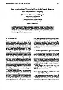
FIG. 3. The maximum transverse Lyapunov exponent l'max as a function of coupling strength a in the Ro¨ssler system.

For any value of a we can calculate the Lyapunov exponents of the variational equation of Eq. ~4!, which is calculated similar to that of Eq. ~2! except that it is three dimensional:

S DS dx' dt dy' dt dz' dt

5

2a

21

1

a

z

0

21

DS D

x' y • ' , z' x2c 0

~6!

where the matrix in Eq. ~6! is the Jacobian of the full Ro¨ssler system plus the coupling term in the x equation. Recall Eq. ~6! gives the dynamics of perturbations transverse to the synchronization manifold. We can use this to calculate the transverse Lyapunov exponents, which will tell us if these perturbations will damp out or not and hence whether the synchronization state is stable or not. We really only need to calculate the largest transverse exponent, since if this is negative it will guarantee the stability of the synchronized state. We call this exponent l'max and it is a function of a. In Fig. 3 we see the dependence of l'max on a. The effect of adding coupling at first is to make l'max decrease. This is common and was shown to occur in most coupling situations for chaotic systems in Ref. 10. Thus, at some intermediate value of a, we will get the two Ro¨ssler systems to synchronize. However, at large a values we see that l'max becomes positive and the synchronous state is no longer stable. This desynchronization was noted in Refs. 10, 21, and 22. At extremely large a we will slave x 2 to x 1 . This is like replacing all occurrences of x 2 in the response with x 1 , i.e. as a →` we asymptotically approach the CR method of synchronization first shown above for the Lorenz systems. Hence, diffusive, one-way coupling and CR are related16 and the asymptotic value of l'max(a→`) tells us whether the CR method will work. Conversely, the asymptotic value of l'max is determined by the stability of the subsystem that remains uncoupled from the drive, as we derived from the CR method.

Chaos, Vol. 7, No. 4, 1997



524

FIG. 5. Chaotic drive and response circuits for a simple chaotic system described by Eqs. ~9!.

FIG. 4. Attractor for the circuit-Ro¨ssler system.

2. Stability for two-way or mutual coupling

Most of the analysis for one-way coupling will carry through for mutual coupling, but there are some differences. First, since the coupling is not one way the Lyapunov exponents of one of the subsystems will not be the same as the exponents for the transverse manifold, as is the case for drive–response coupling. Thus, to be sure we are looking at the right exponents we should always transform to coordinates in which the transverse manifold has its own equations of motion. Then we can investigate these for stability: dx 1 52 ~ y 1 1z 1 ! 1 a ~ x 2 2x 1 ! , dt

dx 2 52 ~ y 2 1z 2 ! dt 1 a ~ x 1 2x 2 ! ,

dy 1 5x 1 1ay 1 , dt

dy 2 5x 2 1ay 2 , dt

dz 1 5b1z 1 ~ x 1 2c ! , dt

dz 2 5b1z 2 ~ x 2 2c ! . dt

~7!

For coupled Ro¨ssler systems like Eq. ~7! we can perform the same transformation as before. Let x' 5x 1 2x 2 , x i 5x 1 1x 2 and with similar definitions for y and z. Then examine the equations for x' , y' , and z' in the limit where these variables are very small. This leads to a variational equation as before, but one that now includes the coupling a little differently:

S DS dx' dt dy' dt dz' dt

5

22 a

21

1

a

z

0

21

DS D

x' y • ' . z' x2c 0

tional equations in which we scale the coupling strength to cover other coupling schemes is much more general than might be expected. We show how it can become a powerful tool later in this paper. The interesting thing that has emerged in the last several years of research is that the two methods we have shown so far for linking chaotic systems to obtain synchronous behavior are far from the only approaches. In the next section we show how one can design several versions of synchronized, chaotic systems. IV. SYNCHRONIZING CHAOTIC SYSTEMS, VARIATIONS ON THEMES A. Simple synchronization circuit

If one drives only a single circuit subsystem to obtain synchronization, as in Fig. 1, then the response system may be completely linear. Linear circuits have been well studied and are easy to match. Figure 5 is a schematic for a simple chaotic driving circuit driving a single linear subsystem.23 This circuit is similar to the circuit that we first used to demonstrate synchronization5 and is based on circuits developed by Newcomb.24 The circuit may be modeled by the equations dx 1 5 a @ 21.35x 1 13.54x 2 17.8g ~ x 2 ! 10.77x 1 # , dt

~9!

dx 2 5 b @ 2x 1 11.35x 2 # . dt ~8!

Note that the coupling now has a factor of 2. However, this is the only difference. Solving Eq. ~6! for Lyapunov exponents for various a values will also give us solutions to Eq. ~8! for coupling values that are doubled. This use of varia-

The function g(x 2 ) is a square hysteresis loop that switches from 23.0 to 3.0 at x 2 522.0 and switches back at x 2 52.0. The time factors are a 5103 and b 5102 . Equation ~9! has two x 1 terms because the second x 1 term is an adjustable damping factor. This factor is used to compensate for the fact that the actual hysteresis function is not a square loop as in the g function. The circuit acts as an unstable oscillator coupled to a hysteretic switching circuit. The amplitudes of x 1 and x 2 will

Chaos, Vol. 7, No. 4, 1997



525

increase until x 2 becomes large enough to cause the hysteretic circuit to switch. After the switching, the increasing oscillation of x 1 and x 2 begins again from a new center. The response circuit in Fig. 5 consists of the x 2 subsystem along with the hysteretic circuit. The x 1 signal from the drive circuit is used as a driving signal. The signals x 82 and x 81 are seen to synchronize with x 2 and x s . In the synchronization, some glitches are seen because the hysteretic circuits in the drive and response do not match exactly. Sudden switching elements, such as those used in this circuit, are not easy to match. The matching of all elements is an important consideration in designing synchronizing circuits, although matching of nonlinear elements often presents the most difficult problem. B. Cascaded drive-response synchronization

Once one views the creation of synchronous, chaotic systems as simply ‘‘linking’’ various systems together, a ‘‘building block’’ approach can be taken to producing other types of synchronous systems. We can quickly build on our original CR scheme and produce an interesting variation that we call a cascaded drive-response system ~see Fig. 8!. Now, provided each response subsystem is stable ~has negative conditional Lyapunov exponents!, both responses will synchronize with the drive and with each other. A potentially useful outcome is that we have reproduced the drive signal x 1 by the synchronized x 3 . Of course, we have x 1 5x 3 only if all systems have the same parameters. If we vary a parameter in the drive, the difference x 1 2x 3 will become nonzero. However, if we vary the responses’ parameters in the same way as the drive, we will keep the null difference. Thus, by varying the response to null the difference, we can follow the internal parameter changes in the drive. If we envision the drive as a transmitter and the response as a receiver, we have a way to communicate changes in internal parameters. We have shown how this will work in specific systems ~e.g., Lorenz! and implemented parameter variation and following in a real set of synchronized, chaotic circuits.6 With cascaded circuits, we are able to reproduce all of the drive signals. It is important in a cascaded response circuit to reproduce all nonlinearities with sufficient accuracy, usually within a few percent, to observe synchronization. Nonlinear elements available for circuits depend on material and device properties, which vary considerably between different devices. To avoid these difficulties we have designed circuits around piecewise linear functions, generated by diodes and op amps. These nonlinear elements ~originally used in analog computers25! are easy to reproduce. Figure 6 shows schematics for drive and response circuits similar to the Ro¨ssler system but using piecewise linear nonlinearities.26 The drive circuit may be described by

FIG. 6. Piecewise linear Ro¨ssler circuits arranged for cascaded synchronization. R15100 kV, R25200 kV, R35R1352 MV, R4575 kV, R5510 kV, R6510 kV, R75100 kV, R8510 kV, R9568 kV, R105150 kV, R115100 kV, R125100 kV, C15C25C350.001 mF, and the diode is a type MV2101.

dz 52 a @ 2g ~ x ! 2z # , dt

H

0, g~ x !5 m x,

~10!

x