guarantee the existence of a diffeomorphism to transform a nonlinear system ..... [14] D. Noh, N. Jo, and H. Seo, âNonlinear observer design by dynamic observer ...
Synchronization of chaotic systems via reduced observers Gang Zheng∗ and Driss Boutat† ∗ INRIA † ENSI
Lille-Nord Europe, 40 Avenue Halley, 59650 Villeneuve d’Ascq, France de Bourges, Institut PRISME, 10, Boulevard Lahitolle 18020 Bourges Cedex, France
Abstract—Synchronization problem of chaotic systems can be seen as an observer design problem. Full order observer needs to estimate the unmeasurable states and the measurable states at the same time, which will increase the complexity. Meanwhile, the reduced observer exhibits some advantages, since it does not need to estimate the measurable outputs. In this paper, a nonlinear canonical form is proposed which permits to design a reduced observer. Sufficient and necessary conditions are given in order to guarantee the existence of a diffeomorphism to transform a nonlinear system into the proposed canonical form. Then a reduced observer for such a canonical form is presented and the simulations illustrate the validity of the proposed method.
I. I NTRODUCTION Since chaotic system is quite sensitive to its parameters and initial conditions, it was thought to be excluded in practice for a long time. After [15] successfully synchronized two identical chaotic systems with different initial conditions, chaos synchronization has been intensively studied in various fields. Since the work of [13], unidirectional synchronization can be viewed as a special case of observer design problem. Many techniques arising from observation theory have been applied to the problem of synchronization, such as observers with linearizable dynamics [8], adaptive [6], generalized hamiltonian form based observers [17], algebraic method [18], [2] or inverse system [5]. However, most of proposed methods are based on the full order observer, which needs to estimate all states of the system, including the measurable states which are the outputs. In order to reduce the complexity of observer design, the so-called reduced observer was proposed, which needs only estimate unmeasurable states of the studied system. It was firstly introduced for linear systems to reduce the number of dynamical equations by estimating only the unmeasurable states. Then it is generalized for nonlinear dynamical systems by imposing the Lipschitz conditions for nonlinear terms [7], [21], [19] and invariant manifold [9]. It is known that the formalism to design nonlinear observer, including reduced observer, for arbitrary nonlinear systems is still missing, hence some researchers tried to solve this problem by introducing the concept of normal form, i.e. transform the nonlinear systems via a diffeomorphism into the normal form, which is easy to design an observer, and then estimate the original states by the inverse of the diffeomorphism. For this technique, reader can refer to [20], [16], [14], [11], [10], [3], [4], [22] and the references
therein. Inspired by this concept, for the problem of synchronization of chaotic systems, this paper proposes a nonlinear canonical form which permits to designe a reduced observer. Sufficient and necessary geometrical conditions are also deduced to determine whether a nonlinear system can be transformed into such a form thought a diffeomorphism. After that a reduced observer is designed for the proposed canonical form. The paper is organized as follows. In section II we give notations, the definition of reduced observer and also the problem statement. Then a nonlinear canonical form is proposed in Section III and Section IV gives necessary and sufficient geometric conditions which allows us to transform a nonlinear system into the proposed nonlinear canonical form. The corresponding reduced observer is studied in Section V and an illustrative example is presented in Section VI. II. N OTATIONS ,
DEFINITIONS AND PROBLEM STATEMENT
Without loss of generality, we assume that the studied chaotic system can be written as follows: x˙ 1 = F1 (x) x˙ 2 = F2 (x) (1) y = x2
where x1 ∈ Rr and x2 ∈ Rp are the states and y ∈ Rp is the measured output, F1 : Rr+p → Rr and F2 : Rr+p → Rp are smooth vector functions. For (1), the following gives the definition of the reduced observer. Definition 1: The dynamical system defined as follows: . x b1 = Fe1 (ˆ x1 , x2 ) where x2 is the output of (1), is a symptomatically reduced observer for (1) if lim k xˆ1 (t) − x1 (t) k= 0.
t→∞
Moreover, it is said to be an exponentially reduced observer if k xˆ1 (t) − x1 (t) k≤ ae−bt k x ˆ1 (0) − x1 (0) k for t > 0, where a, b are both positive constants.
Let recall the famous result of reduced observer for linear systems. For the following system: x˙ 1 = A11 x1 + A12 x2 x˙ 2 = A21 x1 + A22 x2 (2) y = x2
A. Nonlinear canonical form Assume that the studied chaotic system can be decomposed into the following form: x˙ = F1 (x, ζ, ϑ) = f (x, ζ, ϑ) ζ˙ = F21 (x, ζ, ϑ) = γ1 (ζ)H(x) + γ2 (ζ, ϑ) ϑ˙ = F22 (x, ζ, ϑ) = ε (x, ζ, ϑ) �T y = ζ T , ϑT
where Aij are decomposition matrices for 1 ≤ i, j ≤ 2, then it is easy to see [12] the following dynamic is a reduced observer for (2): x ˆ˙ 1 = A11 x ˆ1 + A12 x2 + K(A21 x1 − A21 x ˆ1 ),
(3)
with A21 x1 = y−A ˙ ˆ1 −x1 22 y. The observation error e = x is determined by the following linear system: e˙ = (A11 − KA21 )e which can be stabilized by the choice of K, provide that the pair (A11 , A21 ) is observable. In fact, the reduced observer can be easily extended for a more generic linear system than (2) in the following form: x˙ = A11 x1 + A12 ζ + A13 ϑ ζ˙ = A x + A ζ + A ϑ 21 1 22 23 ˙ = µ (x, ζ, ϑ) ϑ �T y = y1T , y2T = (ζ T , ϑT )T
where y2 = ϑ is another possible measured output, but a redundant one. With those two outputs, the reduced observer (3) can be still applied without taking into account the dynamic ϑ˙ = µ (x, ζ, ϑ). Moreover this dynamic can be used to improve the robustness of the observation. It is well-known that to design a reduced observer directly for nonlinear systems is still an open problem, however this paper tries to solve this problem from another point of view: we introduce a nonlinear canonical form which enables to design a reduced observer, in such a way if a nonlinear system can be transformed into such a nonlinear canonical form, then we can design a reduced observer for this nonlinear system. Consequently this paper deals with the following problems: •
•
•
What is the canonical form which enables to design a reduced observer? What are the sufficient and necessary conditions to transform a nonlinear system (chaotic system) to such a canonical form? How to design a reduced observer for the proposed canonical form?
III. C ANONICAL
FORM FOR REDUCED OBSERVER
In what follows, we will present first the nonlinear canonical form which will be studied in this paper, then the sufficient and necessary geometric conditions to transform a generic chaotic system to such an observable nonlinear canonical form will be analyzed. An exponentially reduced observer can be easily designed for the proposed nonlinear canonical form, which will be detailed in the next section.
(4) (5) (6) (7)
where x ∈ Rr , ζ ∈ R, ϑ ∈ Rp , y ∈ Rp+1 , f : Rr+p+1 → Rr , H ∈ R, γ1 ∈ R and γ2 ∈ R. Moreover, it is assumed that (4-7) is observable and (4) is observable with respective to H (x), which implies that the following 1-formes: θi = dLi−1 (8) f H for 1 ≤ i ≤ r are independent. Then, consider the following observable nonlinear canonical form: z˙ = Az + β(y1 )zr + ρ(y) ξ˙ = α1 (y1 )zr + α2 (y) (9) η˙ = µ (z, y) � � T T = ξ T , ηT y = y1T , y2T where
and
z = (z1 , · · · , zr )T ∈ Rr β = (β1 , · · · , βr )T ∈ Rr ρ = (ρ1 , · · · , ρr )T ∈ Rr η = (η1 , · · · , ηp )T ∈ Rp ξ ∈ R, α1 ∈ R, α2 ∈ R
0 1 .. .
A= 0 0
··· ··· .. .
0 0 .. .
··· ···
1 0
0 0 ··· 0 1
0 0 .. .
0 0
with zr = Cz and C = (0, · · · , 0, 1). Remark 1: Since the nonlinear canonical form (9) is supposed to be observable, thus zr in (9) can be observed from the output y1 , which implies α1 (y) 6= 0. In section V we will see that a reduced observer can be designed for the proposed canonical form (9). Thus the following sub section concerns the deduction of sufficient and necessary conditions in order to transform (4-7) into (9). IV. S UFFICIENT
AND NECESSARY CONDITIONS FOR
THE EXISTENCE OF A DIFFEOMORPHISM
This section is devoted to seeking necessary and sufficient geometric conditions which allows us to transform (4-7) into the proposed nonlinear canonical form (9). For (4-7), denote �T F = f T , F2T � T T T F2 = F21 , F22
and the decomposition of F2 into F21 and F22 makes γ1 (ζ) 6= 0.
After having defined θi for 1 ≤ i ≤ r in (8), then define the vector field τ1 according to the following equations: θj (τ1 ) = 0, θr (τ1 ) = 1
for 1 ≤ j ≤ r − 1
(10)
By induction, we can define the family of vector fields τj as follows: τj = [τj−1 , f ] for 2 ≤ j ≤ r. As we will see, the existence of a diffeomorphism necessarily implies that all τi commutes with each other, i.e. [τi , τj ] = 0 for 1 ≤ i ≤ r and 1 ≤ j ≤ r. We suppose that this condition is satisfied, and assume that σ, ν1 , · · · , νp are the vector fields determined by the following equations: 1) [τi , τj ] = [τi , σ] = [τi , νl ] = [σ, νl ] = [νl , νs ] = 0 for 1 ≤ i, j ≤ r and 1 ≤ l, s ≤ p; 2) dζ(σ) = 1 and dϑ(σ) = 0; 3) dζ(νj ) = 0 and dϑi (νj ) = δij for 1 ≤ i, j ≤ p where δij represents Kronecker delta, i.e. δik = 1 if i = k, otherwise δik = 0. Set θ τ
= =
thus, we can calculate vector fields σ and υ1 , · · · , υp , such that {τi , σ, υl } forms a basis, satisfying the equations mentioned above. Following the same principle, we have
T
(θ1 , · · · , θr , dζ, dϑ1 , · · · , dϑp ) T
(τ1 , · · · , τr , σ, ν1 , · · · , νp )
and denote Λ = θ(τi , σ, νj ) for 1 ≤ i ≤ r and 1 ≤ j ≤ p the evaluation of θ over τ . Due to the observability property, Λ is invertible, hence we can define the following multi 1-forms � � ω1 −1 ω=Λ θ= (11) ω2 where ω2 = (dζ, dϑ1 , · · · , dϑp )T and ω1 is the rest of ω. Then we are ready to state our main result. Theorem 1: There exists a diffeomorphism (z T , ξ T , η T ) = φ(x, ζ, ϑ) which transforms the dynamical system (4-7) into the nonlinear canonical form (9) if and only if the following conditions are satisfied: 1) [τi , τj ] = 0, for 1 ≤ i ≤ r and 1 ≤ j ≤ r; 2) [τr , F¯ ] = V (y1 ) is a vector field which only depends on y1 modulo the sub space spanned by {τi , σ} for 1 ≤ i ≤ r; 3) [τj , F2 ] ∈ ker ω1 for 1 ≤ j ≤ r − 1. � Proof: Necessity: Indeed, if (4-7) can be transformed into (9) via the diffeomorphism (z T , ξ T , η T ) = ∂ ∂ and for 1 ≤ i ≤ r, σ = ∂ξ φ(x, ζ, ϑ), then τi = ∂z i ∂ υl = ∂ϑl for 1 ≤ l ≤ p. And it is easy to check that all conditions of Theorem 1 are satisfied. Sufficiency: Consider the multi 1-forms ω defined in (11), we have ω(τ ) = I(r+p+1)×(r+p+1) , which implies ω(τi ) for 1 ≤ i ≤ r, ω(σ) and ω(υl ) for 1 ≤ l ≤ p are constant. Therefore, dω(τi , τk ) = Lτi ω(τk ) − Lτk ω(τi ) − ω([τi , τk ]) = −ω([τi , τk ])
dω(τi , σk ) = −ω([τi , σk ]), dω(τi , υl ) = −ω([τi , υl ]) dω(υl , υt ) = −ω([υl , υt ]) Since ω is an isomorphism, this implies the equivalence between [τi , τk ] = [τi , σ] = [τi , νl ] = [σ, νl ] = [νl , νt ] = 0 and dω = 0 According to theorem of Poincar´e [1], dω = 0 implies that there exists a local diffeomorphism (z T , ξ T , η T ) = φ(x, ζ, ϑ) such that ω = dφ. We note ωi = dφi for 1 ≤ i ≤ 2. Since condition (1) in Theorem 1 is satisfied and τ ∂ ∂ and , φ∗ (σ) = ∂ζ is a basis, it implies φ∗ (τi ) = ∂z i ∂ φ∗ (υl ) = ∂ϑl for 1 ≤ i ≤ r and 1 ≤ l ≤ p. Now let us clarify the affect of this transformation on f (x, ζ, ϑ) definedin (4). By the diffeomorphism z˙ φ(x, ζ, ϑ), we have ξ˙ = φ∗ (F ) where F = η˙ � � f . It is easy to see that F2 � � � � � � ω1 (f + F2 ) ω1 (f ) + ω1 (F2 ) f = = ω ω2 (f + F2 ) ω2 (f ) + ω2 (F2 ) F2 Then, for 1 ≤ i ≤ r, � ∂ (φ∗ (F )) = ∂zi � = � =
we get [ω1 (τi ) , ω1 (f ) + ω1 (F2 )] [ω2 (τi ) , ω2 (f ) + ω2 (F2 )] � ω1 [τi , f ] + ω1 [τi , F2 ] [ω2 τi , ω2 (f ) + ω2 (F2 )] ∂ ∂zi+1
[ω2 (τi ) , ω2 (f ) + ω2 (F2 )]
� �
since condition (3) [τi , F2 ] ∈ ker ω1 for 1 ≤ i ≤ r − 1 implies ω1 [τi , F2 ] = 0. By integrating we obtain: ω1 (F ) = Az + ̺(y, zr ). Moreover, as we know ∂ ∂zk H
◦ φ−1
= dH(τk ) = θ1 (τk )
then according to the definition of τ1 in (10), we get ∂ H ◦ φ−1 = 1 ∂zr which implies (5) can be written as ζ˙ = γ1 (ζ)zr + γ2 (ζ)
(12)
Hence, by setting ω2 = dφ2 where φ2 = I(p+1)×(p+1) , then we get Az + ̺(y, zr ) φ∗ (F ) = γ1 (y1 )zr + γ2 (y) (13) µ (z, ξ, η)
Finally, by the condition (2), we have � �� ∂φ∗ (F¯ ) = φ∗ � τr , F¯ ∂zr � Pr V (y )τ + W (y )σ = φ∗ j 1 j 1 Pr j=1 ∂ = j=1 Vj (y1 ) ∂z∂ j + W (y1 ) ∂ξ
to overcome this problem, we introduced an algebraic estimator as follows:
where Γ(y1 ) =
which means W (y1 ) = α1 (y1 ) and ̺(y, zr ) in (12) can be decomposed as: ̺(y, zr ) = β(y1 )zr + ρ(y) Thus we proved that (4-7) can be transformed to (9) via φ. V. R EDUCED
OBSERVER DESIGN FOR THE CANONICAL FORM
If Theorem 1 is satisfied, then (4-7) can be transformed into (9) by a diffeomorphism (z T , ξ T , η T ) = φ(x, ζ, ϑ). This section is devoted to designing a reduced observer for the deduced nonlinear canonical form. Once the states of the canonical form have been estimated, by the inverse of the diffeomorphism, we can then recover the states of original chaotic system in the form of (4-7). First of all, for (9) if we can accurately measure y1 , y2 and calculate y˙ 1 , this allows us to define a ”new” output Y being a function of known output y and the derivative of y1 in (9): Y = α−1 1 (y1 ) (y˙ 1 − α2 (y))
(14)
(15)
where K(y1 ) = −β(y1 ) + κ and Y is defined in (14), is an exponentially reduced observer for (9), if the chosen κ makes (A + κC) Hurwitz. Proof: Let e = zˆ − z be the estimation error. Since zr = Cz, then we can easily derive the dynamic of observation error from (9) and (15) as follows e˙ = [A + (β(y1 ) + K(y1 ))C]e
ς = zˆ + Γ(y1 )
(18)
K(y1 )α−1 1 (y1 )dy1 .
Remark 2: It should be noted that Γ(y1 ) defined above can be considered as a signal of filtered y1 , and thus limit the influence of noise on y1 . Inserting Y defined in (14) into (15), (15) is rewritten into zˆ˙ + K(y1 )α−1 (y1 )y˙ 1 = (A + β(y1 )C + K(y1 )C)ˆ z 1
+ρ(y) + K(y1 )α−1 1 (y1 )α2 (y) (19) In order to avoid the derivative of y1 , we take the new variable ς into account, then a more practical reduced observer can be derived from (19) as follows ς˙ =
(A + β(y1 )C + K(y1 )C) (ς − Γ(y1 )) +ρ(y) + K(y1 )α−1 1 (y1 )α2 (y1 ) (A + κC)ς + ρ(y) − (A + κC)Γ(y1 ) +K(y1 )α−1 1 (y1 )α2 (y)
=
(20)
with Γ(y1 ) defined in (18). The proof of the convergence of ς − Γ(y1 ) in (20) to z of the canonical form (9) is evident, and then one can estimate x of (4-7) by φ−1 . The next section gives an example to illustrate the feasibility of the proposed method. VI. I LLUSTRATIVE EXAMPLE
Then we have the following preliminary result. Proposition 1: The following dynamical system: zˆ˙ = Aˆ z + β(y1 )C zˆ + ρ(y) − K(y1 )(Y − C zˆ)
R
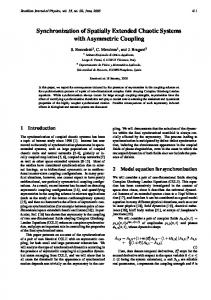
In order to highlight the proposed method in this paper, let consider the well-known R¨ossler chaotic system as follows: x˙ 1 = x2 + ax1 x˙ 2 = −x1 − x3 (21) x˙ 3 = c + x3 (x2 − b) y = x3 with a = c = 0.2, b = 5.7. Fig. 1 depicts the chaotic attractor of R¨ossler system when a = c = 0.2, b = 5.7.
(16) 10
Since the gain matrix K(y1 ) can be freely chosen, hence without loss of generality we set
z
1
ς + 3logy
8
1
e˙ = (A + κC)e.
(17)
Consequently, if κ is chosen in such a way that matrix (A + κC) is Hurwitz, then the exponential convergence of zˆ to z can be guaranteed. Let us remark that the proposed reduced observer (15) is based on the ”new” output Y defined in (14), which clearly shows that the derivative of the real output y1 should be calculated according to (14). However, it is well-known that the derivative of noisy signal should be avoided if possible in practice, since derivative operation will amplify the influence of noise. Hence, in order
4 2 0
1
which makes (16) become
z and its estimate
6
K(y1 ) = −β(y1 ) + κ
−2 −4 −6 −8
0
5
10 t (s)
15
20
Fig. 1. Phase portrait of R¨ossler chaotic system with initial conditions x1 (0) = −0.8, x2 (0) = −1 and x3 (0) = 1.
By setting x=
�
x1 x2
�
, ζ = x3
we can rewrite (21) into the following form: � � � � x˙ 1 x2 + ax1 x˙ = = x˙ 2 −x1 − ζ ˙ = c + ζ (x2 − b) ζ y=ζ
(22)
We can then design a reduced observer for (23). Following the conditions of Proposition 1, one can find the gain � � −4 κ= −4 such that A + κC has two equal eigenvalues −2. Then one obtains � � � � 1 ∂Γ −3 −3 = K (y) = and −a − 4 −a − 4 ∂y y
which is of the form (4-6) with
H (x)� = x2 � x2 + ax1 f= −x1 − ς F2 = c + ς (x2 − b) �T F¯ = f T , F2T
which yields
Then we can define the following 1-forms:
Γ (y) =
θ1 = dx2 , θ2 = −dx1 − dx3 and dζ = dx3
−3 −a − 4
�
ln y
Thus, according to Proposition 1, the reduced observer for (23) can be designed as follows:
which yields τ1 = −
�
∂ ∂ ∂ ∂ , τ2 = −a + and σ = ∂x1 ∂x1 ∂x2 ∂x3
.
It is easy to check that [τ1 , τ2 ] = 0 and [τi , σ] = 0 for 1 ≤ i ≤ 2. Moreover we have: � ∂ ∂ ∂ [τ2 , F¯ ] = 1 − a2 +a + x3 ∂x1 ∂x2 ∂x3 = −τ1 + aτ2 + x3 σ1 In order to calculate the diffeomorphism, let compute: 0 1 0 Λ = θτ = 1 a −1 0 0 1 and it yields
−1 −a 0 1 0 ω = Λ−1 θ = 0 0 0 1 � � −x1 − ax2 . which gives ω1 = x2 Then one can check that
zˆ1 = −ˆ z2 + az3 + 3 (z2 − zˆ2 ) . zˆ2 = zˆ1 + aˆ z2 − z3 + (a + 4) (z2 − zˆ2 ) where z2 = (y˙ + by − c) /y, which explicitly depends on the derivative of y. Since the derivative of the output will amplify the influence of noise, so in order to overcome this problem, let introduce the following algebraic estimator: � � −3 ς = zˆ + Γ = zˆ + ln y −a − 4 Then, after a straightforward calculation, one has the following reduced observer for (23) in the coordinate of ς: .
ςˆ1 = −4ˆ ς2 + ay + (4a + 16) ln y − 3 (c − by) /y . ςˆ2 = ςˆ1 − 4ˆ ς2 − y + (4a + 13) ln y − (a + 4) (c − by) /y
ω1 [τ1 , F2 ] = 0 implying [τ1 , F2 ] ∈ ker ω1 . Thus all conditions of Theorem 1 are satisfied, and one deduces the following diffeomorphism:
Fig. 2-7 are the simulations of the obtained reduced observer for (23), and it is shown that the deduced observer can perfectly estimate the unmeasurable states without estimating the output. 25 z
T
T
φ = (z1 , z2 , ξ) = (−x1 − ax2 , x2 , ζ)
which is in the proposed normal form (9) with � � � � 0 0 −1 A= ,β = a � 1 0� aξ ρ= , C = (0, 1) −ξ α1 = y, α2 = c − by
1
1
15
1
z and ς
which transforms (21) into z˙1 = −z2 + aξ z˙ = z + az − ξ 2 1 2 ξ˙ = z2 ξ + c − bξ y=ξ
1
ς
20
(23)
10
5
0
−5
−10
0
5
10 t (s)
15
20
Fig. 2. z1 and the estimate of ς1 with initial conditions z1 (0) = 1 and ς1 (0) = 0.
20
8 z
z
2
2
ς2
15
ς2 + (a+4)logy
6 4
z and ς
2
z and its estimate
10
0 −2
2
2
5
2
0
−4 −6
−5 −8 −10
0
5
10 t (s)
15
−10
20
Fig. 3. z2 and the estimate of ς2 with initial conditions z2 (0) = −1 and ς2 (0) = 0.
5
10 t (s)
15
20
Fig. 5. z2 and its estimate with initial conditions z2 (0) = −1 and zˆ2 (0) = ς2 (0) = 0.
10
8 z
x
1
ς + 3logy
8
6
1
4
4
2
x and its estimate
6
2 0
1
estimate
0 −2
1
1
z and its estimate
0
−2 −4
−4 −6
−6
−8
−8
−10
0
5
10 t (s)
15
20
Fig. 4. z1 and its estimate with initial conditions z1 (0) = 1 and zˆ1 (0) = ς1 (0) = 0.
VII. C ONCLUSION The synchronization problem of chaotic systems via reduced observer is studied in this paper. We proposed a new canonical form which enables to design a reduced observer. Sufficient and necessary conditions are given to determine whether a chaotic nonlinear system can be transformed into such a form. Then a reduced observer is studied for the proposed canonical form, and the feasibility is highlighted by an example. R EFERENCES [1] R. Abraham and J. E. Marsden, “Foundation of mechanics,” Princeton, New Jersey, 1966. [2] J.-P. Barbot, M. Fliess, and T. Floquet, “An algebraic framework for the design of nonlinear observers with unknown inputs,” IEEE Conference on Decision and Control, pp. 384–389, 2007. [3] D. Bestle and M. Zeitz, “Canonical form observer design for nonlinear time variable systems,” International Journal of Control, vol. 38, pp. 419–431, 1983. [4] D. Boutat, A. Benali, H. Hammouri, and K. Busawon, “New algorithm for observer error linearization with a diffeomorphism on the outputs,” Automatica, vol. 45, pp. 2187–2193, 2009. [5] U. Feldmann, M. Hasler, and W. Schwarz, “Communication by chaotic signals: The inverse system approach,” International Journal of Cricuit Theory and Applications, vol. 24, pp. 551–576, 1996. [6] A. Fradkov, H. Nijmeijer, and A. Markov, “Adaptive observerbased synchronization for communication,” International Journal of Bifurcation and Chaos, vol. 10, pp. 2807–2813, 2000. [7] W. M. Haddad and D. S. Bernstein, “Optimal reduced-order observer-estimators,” in Proceedings of the 28th IEEE Conference on Decision and Control, 1989.
0
5
10 t (s)
15
20
Fig. 6. x1 and its estimate with initial conditions x1 (0) = −1 and x ˆ1 (0) = −ˆ z1 (0) − aˆ z2 (0) = 0.
[8] H. Huijberts, T. Lilge, and H. Nijmeijer, “Nonlinear discrete-time synchronization via extended observers,” International Journal of Bifurcation and Chaos, vol. 11, no. 7, pp. 1997–2006, 2001. [9] D. Karagiannis, D. Carnevale, and A. Astolfi, “Invariant manifold based reduced-order observer design for nonlinear system,” IEEE Transactions on Automatic Control, vol. 53, no. 11, pp. 2602– 2614, 2008. [10] A. Krener and A. Isidori, “Linearization by output injection and nonlinear observer,” Systems & Control Letters, vol. 3, pp. 47–52, 1983. [11] A. Krener and W. Respondek, “Nonlinear observer with linearizable error dynamics,” SIAM Journal of Control and Optimization, vol. 30, pp. 197–216, 1985. [12] D. Leunberger, “An introduction to the observers,” IEEE Transactions on Automatica Control, vol. 16, no. 6, pp. 596–602, 1971. [13] H. Nijmeijer and I. Mareels, “An observer looks at synchronization,” IEEE Transactions on Circuits and Systems-1: Fundamental theory and Applications, vol. 44, no. 10, pp. 882–891, 1997. [14] D. Noh, N. Jo, and H. Seo, “Nonlinear observer design by dynamic observer error linearization,” IEEE Transactions on Automatica Control, vol. 49, 2004. [15] L. Pecora and T. Carroll, “Synchronization in chaotic systems,” Physical Review Letters, vol. 64, no. 8, pp. 821–824, 1990. [16] W. Respondek, A. Pogromsky, and H. Nijmeijer, “Time scaling for observer design with linearization error dynamics,” Automatica, vol. 40, no. 2, pp. 277–285, 2004. [17] H. Sira-Ramirez and C. Cruz-Hernandez, “Synchronization of chaotic systems: a generalized hamiltonian approach,” International Journal of Bifurcation and Chaos, vol. 11, no. 5, pp. 1381– 1395, 2001. [18] H. Sira-Ramirez and M. Fliess, “An algebraic state estimation approach for the recovery of chaotically encrypted messages,” International Journal of Bifurcation and Chaos, vol. 16, no. 2, pp. 295–309, 2006. [19] V. Sundarpandian, “Reduced order observer design for nonlinear
8 x2 6
estimate
2 0 −2
2
x and its estimate
4
−4 −6 −8 −10
0
5
10 t (s)
15
20
Fig. 7. x2 and its estimate with initial conditions x2 (0) = −1 and x ˆ2 (0) = zˆ2 (0) = 0.
systems,” Applied mathematics letters, vol. 19, no. 9, pp. 936–941, 2006. [20] X. Xia and W. Gao, “Nonlinear observer with linearizable error dynamics,” SIAM Journal of Control and Optimization, vol. 27, pp. 199–216, 1989. [21] M. Xu, “Reduced-order observer design for one-sided lipschitz nonlinear systems,” IMA Journal of Mathematical Control and Information, vol. 26, no. 3, pp. 299–317, 2009. [22] G. Zheng, D. Boutat, and J.-P. Barbot, “Signal output dependent observability normal form,” SIAM Journal of Control and Optimization, vol. 46, no. 6, pp. 2242–2255, 2006.