In the Name of Allah, Most Gracious, and Most Merciful,. To my parents ... I would like to thank my advisor, Professor Earl E. Swartzlander, Jr. for his guidance ...
Copyright by Hani Hasan Mustafa Saleh 2009
The Dissertation Committee of Hani Hasan Mustafa Saleh certifies that this is the approved version of the following dissertation:
Fused Floating-Point Arithmetic For DSP
Committee:
____________________________________ Earl E. Swartzlander, Jr., Supervisor ____________________________________ Mircea Driga ____________________________________ Mohamed Gouda ____________________________________ Michael Orshansky ____________________________________ Nur Touba
Fused Floating-Point Arithmetic For DSP
by Hani Hasan Mustafa Saleh, B.S.; M.S.
Dissertation Presented to the Faculty of the Graduate School of the University of Texas at Austin in Partial Fulfillment of the Requirements for the Degree of Doctor of Philosophy
The University of Texas at Austin May, 2009
In the Name of Allah, Most Gracious, and Most Merciful, To my parents, my wife, my children and all of my six brothers.
Acknowledgements First, I want to thank Allah (Arabic for the God) for providing me the will, the time and the energy to accomplish this work. I am grateful to my mother for guiding my steps on the path of achievements since my infanthood, my father for raising me up and being my model till his last breath, my brothers Yousef, Rami, Ali, Suleiman, Mohammad and Mutei for taking care of me and supporting me always, my children Shushu, Yousuf and Yahya for their love and support and special thanks and gratitude to my beloved wife Eman for her love, support, and patience during the course of this work; I really appreciate the sacrifice that my wife and children made to facilitate this work and their prayers throughout this endeavor. I would like to thank my advisor, Professor Earl E. Swartzlander, Jr. for his guidance, understanding and support throughout the course of this research. Working with him has been a great experience and great fun. Thanks to my committee members for their ideas and invaluable feedback. I would like also to thank Professor Adnan Aziz for his guidance and support. Thanks to the Electrical and Computer Engineering staff for their assistance. I would like to express my gratitude to my colleagues at the University of Texas at Austin, Bassam Mohammad and Baker Mohammad, as well as special thanks to my colleagues while I was at University of Texas at San Antonio for their encouragement and assistance; special thanks to Adnan Suleiman, Adel Husain, Amjad Odetallah, Khaldoun Batyneh, and Hassan Ali. Also, special thanks to my proofreaders Akif Ali, Athar Tayyeb, Baker Mohammad, Bryan Dobbs, Dan Cermak, Jonathan Tong, Scott Holmes, Richard Umberhocker, Clay Douglass, Stephan Kulik, III and Paul Adeleke, for great feedback, as well as special thanks to Khader Mohammad for his assistance with the backend tools and libraries. In addition, special thanks to my colleagues and managers at my current and previous places of employment for their understanding and encouragement.
v
Finally, I am indebted to my colleagues at my previous place of employment, Carl Lemonds, Dimitri Tan and Eric Quinnell, for all the knowledge they shared with me about floating-point hardware design.
vi
Fused Floating-Point Arithmetic for DSP
Publication No. _____________________
Hani Hasan Mustafa Saleh, Ph.D. The University of Texas at Austin, 2009 Supervisor: Earl E. Swartzlander, Jr.
Floating-point arithmetic is attractive for the implementation for a variety of Digital Signal Processing (DSP) applications because it allows the designer and user to concentrate on the algorithms and architecture without worrying about numerical issues. In the past, many DSP applications used fixed point arithmetic due to the high cost (in delay, silicon area, and power consumption) of floating-point arithmetic units. In the realization of modern general purpose processors, fused floating-point multiply add units have become attractive since their delay and silicon area is often less than that of a discrete floating-point multiplier followed by a floating point adder. Further the accuracy is improved by the fused implementation since rounding is performed only once (after the multiplication and addition). This work extends the consideration of fused floating-point arithmetic to operations that are frequently encountered in DSP. The Fast Fourier Transform is a case in point since it uses a complex butterfly operation. For a radix-2 implementation, the butterfly consists of a complex multiply and the complex addition and subtraction of the same pair of data. For a radix-4 implementation, the butterfly consists of three complex multiplications and eight complex additions and subtractions. Both of these butterfly
vii
operations can be implemented with two fused primitives, a fused two-term dot-product unit and a fused add-subtract unit. The fused two-term dot-product multiplies two sets of operands and adds the products as a single operation. The two products do not need to be rounded (only the sum is normalized and rounded) which reduces the delay by about 15% while reducing the silicon area by about 33%. For the add-subtract unit, much of the complexity of a discrete implementation comes from the need to compare the operand exponents and align the significands prior to the add and the subtract operations. For the fused implementation, sharing the comparison and alignment greatly reduces the complexity. The delay and the arithmetic results are the same as if the operations are performed in the conventional manner with a floating-point adder and a separate floating-point subtracter. In this case, the fused implementation is about 20% smaller than the discrete equivalent.
viii
Table of Contents Acknowledgements.............................................................................................. v Fused Floating-Point Arithmetic for DSP......................................................... vii Table of Contents ................................................................................................ ix List of Figures..................................................................................................... xii List of Tables ...................................................................................................... xv Chapter 1
Introduction ...................................................................................... 1
1.1 Motivation..................................................................................................................................1 1.2 Problem Description ..................................................................................................................2 1.3 Dissertation Overview ...............................................................................................................4
Chapter 2
Background ...................................................................................... 5
2.1 Computer Arithmetic Overview ................................................................................................5 2.2 Fixed-Point Representation Overview and Implementation Issues ...........................................5 2.2.1. Fixed-Point Precision Loss and Overflow.................................................................6 2.3 An Overview of the IEEE-754 Floating-Point Standard ...........................................................7 2.4 An Overview of the Floating-Point Fused Multiply-Add (FMA) Operation [14] .....................9 2.5 Other Fused Arithmetic Units..................................................................................................10 2.6 The Fast Fourier Transform (FFT) Algorithm.........................................................................11 2.7 Summary ..................................................................................................................................13
Chapter 3
Research Approach and Design Methodology............................ 14
3.1 3.2 3.3 3.4 3.5 3.6
Research Approach ..................................................................................................................14 High-Level Modeling...............................................................................................................16 RTL Digital Design Using Verilog HDL.................................................................................17 The EDA Tools Used in The ASIC Implementation Flow ......................................................18 Functional Verification Using Simulation ...............................................................................20 ASIC Implementation Flow.....................................................................................................21 3.6.1. Dynamic Power Estimation Detailed Methodology ................................................28 3.7 The 45nm CMOS Technology Process Used to Implement the Primitive and the Derived Units ...........................................................................................................................30 3.8 Notes About ASIC Standard-Cell Libraries and ASIC Flows ................................................31
Chapter 4
Floating-Point Fused Add-Subtract Unit ...................................... 33
4.1 Introduction..............................................................................................................................33 4.2 Floating-Point Adder Design ...................................................................................................34 4.2.1. Basic Floating-Point Addition Algorithm ...............................................................34 4.3 Fused Add-Subtract Unit Design Approachs...........................................................................37 4.4 Implementation Results ...........................................................................................................40 4.4.1. Floating-Point Adder (FPA) Unit ............................................................................40
ix
4.4.1.1. Timing ..............................................................................................44 4.4.1.2. Place and Route Results ...................................................................44 4.4.1.3. Power and Energy Estimation Results..............................................47 4.4.2. Serial Add-Subtract (Serial AS) Unit ......................................................................47 4.4.2.1. Timing ..............................................................................................48 4.4.2.2. Place and Route Results ...................................................................49 4.4.2.3. Power and Energy Estimation Results..............................................52 4.4.3. Parallel Add-Subtract (Parallel AS) Unit ................................................................52 4.4.3.1. Timing ..............................................................................................52 4.4.3.2. Place and Route Results ...................................................................53 4.4.3.3. Power and Energy Estimation Results..............................................56 4.4.4. Fused Add-Subtract (Fused AS) Unit......................................................................56 4.4.4.1. Timing ..............................................................................................56 4.4.4.2. Place and Route Results ...................................................................57 4.4.4.3. Power and Energy Estimation Results..............................................60 4.5 Add-Subtract Unit Implementation Results Summary ............................................................61
Chapter 5
Floating-Point Fused Two-Term Dot-Product Unit...................... 65
5.1 Introduction..............................................................................................................................65 5.2 Floating-Point Multiplier Design .............................................................................................68 5.2.1. Basic Floating-Point Multiplier Algorithm .............................................................69 5.3 Fused DP Unit Design Approach.............................................................................................71 5.4 Dot-Product Unit Implementation Results...............................................................................76 5.4.1. Floating-point Multiplier (FPM) Unit .....................................................................77 5.4.1.1. Timing ..............................................................................................79 5.4.1.2. Place and Route Results ...................................................................80 5.4.1.3. Power and Energy Estimation Results..............................................83 5.4.2. Floating-point Two-Term Serial Dot-Product (Serial DP) Unit..............................84 5.4.2.1. Timing ..............................................................................................85 5.4.2.2. Serial DP Place and Route Results ...................................................85 5.4.2.3. Power and Energy Estimation Results..............................................88 5.4.3. Floating-point Two-Term Parallel Dot-Product (Parallel DP) Unit ........................88 5.4.3.1. Timing ..............................................................................................88 5.4.3.2. Place and Route Results ...................................................................89 5.4.3.3. Power and Energy Estimation Results..............................................91 5.4.4. Floating-point Two-Term Fused Dot-Product (Fused DP) Unit .............................91 5.4.4.1. Timing ..............................................................................................91 5.4.4.2. Place and Route Results ...................................................................92 5.4.4.3. Power and Energy Estimation Results..............................................95 5.5 Dot-Product Unit Implementation Results Summary ..............................................................96
Chapter 6
Floating-Point Fused Radix-2 and Radix-4 FFT Butterfly Units102
6.1 Radix-2 FFT Butterfly ...........................................................................................................102 6.1.1. Radix-2 Butterfly Design Approach......................................................................103 6.2 Radix-4 FFT Butterfly ...........................................................................................................105
x
6.3 Butterfly Unit Implementation Results ..................................................................................108 6.3.1. Floating-point Discrete Parallel Radix-2 FFT Butterfly........................................109 6.3.1.1. Timing ............................................................................................109 6.3.1.2. Place and Route Results .................................................................110 6.3.1.3. Power and Energy Estimation Results............................................113 6.3.2. Floating-point Fused Radix-2 FFT Butterfly Unit.................................................114 6.3.2.1. Timing ............................................................................................114 6.3.2.2. Place and Route Results .................................................................114 6.3.2.3. Power and Energy Estimation Results............................................117 6.3.3. Floating-point Discrete Parallel Radix-4 FFT Butterfly Unit................................117 6.3.3.1. Timing ............................................................................................118 6.3.3.2. Place and Route Results .................................................................118 6.3.3.3. Power and Energy Estimation Results............................................121 6.3.4. Floating-point Fused Radix-4 FFT Butterfly.........................................................122 6.3.4.1. Timing ............................................................................................122 6.3.4.2. Place and Route Results .................................................................123 6.3.4.3. Power and Energy Estimation Results............................................125 6.4 Butterfly Unit Implementation Results Summary .................................................................126 6.5 Butterfly Unit Error Analysis.................................................................................................131
Chapter 7
Conclusion.................................................................................... 138
7.1 The Key Contributions...........................................................................................................138 7.2 Future Research .....................................................................................................................144
Bibliography ..................................................................................................... 145 VITA ................................................................................................................... 149
xi
List of Figures Figure 1. FFT Spectrum Calculation Using: Double Precision Floating-Point, Single Precision Floating-Point and 12-bit Fixed-Point Without and With Scaling Figure 2. Block Diagram of a Floating-point Fused Multiply-add Unit, reduced from [14] Figure 3. Radix-2 Butterflies Figure 4. 8-point Radix-2 DIT FFT Figure 5. 8-point Radix-2 DIF FFT Figure 6. Research Flow Figure 7. Verilog HDL for a 2:1 Multiplexer Figure 8. Functional Verification Using Simulation Figure 9. Implementation Sub-Flow Figure 10. Analysis Sub-Flow Figure 11. The Floating-Point Fused Add-Subtract Unit Concept Figure 12. A Conventional Floating-Point Adder Figure 13. Conventional Parallel Realization of an Add-Subtract Unit Figure 14. Conventional Serial Realization of an Add-Subtract Unit Figure 15. Floating-Point Fused Add-Subtract Unit Figure 16. Align Circuit Figure 17. Significand Adder Circuit Figure 18. Normalization Circuit Figure 19. Rounding Circuit Figure 20. Finalization Circuit Figure 21. Floating-Point Adder Unit Routing Figure 22. Floating-Point Adder Unit Placement with the Critical Timing Path Highlighted Figure 23. Serial AS Micro-Architecture Figure 24. Serial AS Unit Routing Figure 25. Serial AS Unit Placement with Critical Path Highlighted Figure 26. Parallel AS Unit Routing Figure 27. Parallel AS Unit Placement with Critical Timing Path Highlighted Figure 28. Fused AS Unit Routing Figure 29. Fused AS Unit Placement with Critical Timing Path Highlighted Figure 30. Add-Subtract Unit Delay Comparison Figure 31. Add-Subtract Unit Area Comparison Figure 32. Add-Subtract Unit Power Consumption Comparison Figure 33. Add-Subtract Unit Energy Consumption Comparison Figure 34. Two-Term Dot-Product Serial Implementation Figure 35. Two-Term Dot-Product Parallel Implementation Figure 36. The Fused DP Unit Concept Figure 37. Complex Multiplier Computation Figure 38. Basic Floating-Point Multiplier Figure 39. Conventional Floating-Point FMA unit [14] Figure 40. Floating-Point Fused Two-Term Dot-Product Unit Figure 41. Floating-Point Fused Multiply-Add Unit Exponent Compare Circuit Figure 42. Floating-Point Fused Two-Term Dot-Product Unit Exponent Compare Circuit Figure 43. LZA Circuit Concept [39]
xii
7 10 12 12 12 15 18 21 24 27 34 37 38 38 39 41 42 42 43 43 45 46 48 50 51 54 55 58 59 61 62 63 64 66 66 67 68 70 72 73 74 75 75
Figure 44. Floating-Point Fused Two-Term Dot-Product Unit Alignment Circuit Figure 45. Radix-8 Booth Significand Multiplier Figure 46. Partial Product Summation Tree (Using One Hot Encoding) Figure 47. FPM Unit Routing Figure 48. FPM Unit Placement with the Critical Timing Path Highlighted Figure 49. Serial DP Micro-Architecture Figure 50. Serial DP Unit Routing Figure 51. Serial DP Unit Placement Figure 52. Parallel DP Unit Routing Figure 53. Parallel DP Unit Routing Figure 54. Fused DP Unit Routing Figure 55. Fused DP Unit Placement Figure 56. Two-Term Dot-Product Unit Delay Comparison Figure 57. Two-Term Dot-Product Unit Area Comparison Figure 58. Two-Term Dot-Product Unit Power Consumption Comparison Figure 59. Two-Term Dot-Product Unit Energy Consumption Comparison Figure 60. Radix-2 FFT Butterfly Unit Concept Figure 61. Parallel Implementation of Radix-2 Decimation in Frequency FFT Butterfly Unit Figure 62. Serial Implementation of Radix-2 Decimation in Frequency FFT Butterfly Unit Figure 63. Fused Radix-2 Decimation in Frequency FFT Butterfly Unit Figure 64 Radix-4 Decimation in Time FFT Butterfly Unit Figure 65 Parallel Implementation of Radix-4 Decimation in Time FFT Butterfly Unit Figure 66 Fused Radix-4 Decimation in Time FFT Butterfly Unit Figure 67. Floating-Point Discrete Parallel Radix-2 FFT Butterfly Unit Routing Figure 68. Floating-Point Discrete Parallel Radix-2 FFT Butterfly Unit Placement Figure 69. Floating-Point Fused Radix-2 Butterfly Unit Routing Figure 70. Floating-Point Fused Radix-2 Butterfly Unit Placement Figure 71. Floating-Point Discrete Parallel Radix-4 FFT Butterfly Unit Routing Figure 72. Floating-Point Discrete Parallel Radix-4 FFT Butterfly Unit Placement Figure 73. Floating-Point Fused Radix-4 Butterfly Unit Routing Figure 74. Floating-Point Fused Radix-4 Butterfly Unit Placement Figure 75. Butterfly Unit Delay Comparison Figure 76. Butterfly Unit Area Comparison Figure 77. Butterfly Unit Power Comparison Figure 78. Butterfly Unit Energy Consumption Comparison Figure 79. Error Analysis Experiments Block Diagram Figure 80. Radix-2 Butterfly Unit Errors Using 64K Random Input Vector Figure 81. Radix-4 Butterfly Unit Errors Using 64K Random Input Vector Figure 82. Radix-2 64K FFT Based on Discrete and Fused Radix-2 Butterflies Errors Using 64K Random Input Vector Figure 83. Radix-4 64K FFT Based on Discrete and Fused Radix-4 Butterflies Errors Using 64K Random Input Vector Figure 84. FFT Butterflies Error Simulation Max and Average Error Figure 85. 64K FFT Error Simulation Max and Average Error Figure 86. Add-Subtract Unit Comparison Figure 87. Two-Term Dot-Product Function Design Options Comparison
xiii
76 78 79 81 82 84 86 87 89 90 93 94 97 98 99 100 102 103 104 105 106 107 108 111 112 115 116 119 120 123 124 127 128 129 130 132 133 134 135 136 137 137 139 140
Figure 88. Radix-2 FFT Butterfly Design Options Comparison Figure 89. Radix-4 FFT Butterfly Design Options Comparison Figure 90. FFT Butterflies Error Simulation Max and Average Error as a Percentage of the Discrete Radix-4 BF Error Figure 91. 64K FFT Error Simulation Max and Average Error as a Percentage of the Discrete Radix-4 FFT Error
xiv
141 142 143 143
List of Tables Table 1. IEEE-754 Storage Layout [1] Table 2. Basic Floating-Point Adder Algorithm Latency Table 3. Floating-Point Adder Critical Timing Path Table 4. Floating-Point Adder Area Distribution Table 5. Floating-Point Adder Total Power Distribution Table 6. Serial AS Critical Timing Path Table 7. Serial AS Area Distribution Table 8. Serial AS Average Power Distribution Table 9. Parallel AS Critical Timing Path Table 10. Parallel AS Area Distribution Table 11. Parallel AS Total Power Distribution Table 12. Fused AS Critical Timing Path Table 13. Fused AS Area Distribution Table 14. Fused AS Average Power Distribution Table 15. Add-Subtract Unit Delay Comparison for Performing Simultaneous Add and Subtract on Two Operands Table 16. Add-Subtract Unit Area Comparison Table 17. Add-Subtract Unit Power Consumption Comparison Table 18. Add-Subtract Unit Energy Consumption Comparison Table 19. Radix-8 Booth Encoding Table Table 20. Floating-Point Multiplier Critical Timing Path Table 21. FPM Area Distribution Table 22. FPM Unit Average Power Distribution Table 23. Serial DP Critical Timing Path Table 24. Serial DP Unit Area Distribution Table 25. Serial DP Power Distribution Table 26. Parallel DP Unit Critical Timing Path Table 27. Parallel DP Area Distribution Table 28. Parallel DP Unit Average Power Distribution Table 29. Fused DP Unit Critical Timing Path Table 30. Fused DP Unit Area Distribution Table 31. Fused DP Unit Power Distribution Table 32. Two-Term Dot-Product Unit Delay Comparison Table 33. Two-Term Dot-Product Unit Area Comparison Table 34. Two-Term Dot-Product Unit Power Consumption Comparison Table 35. Two-Term Dot-Product Unit Energy Consumption Comparison Table 36. Floating-Point Discrete Parallel Radix-2 FFT Butterfly Critical Timing Path Table 37. Floating-Point Discrete Parallel Radix-2 FFT Butterfly Unit Area Distribution Table 38. Floating-Point Discrete Parallel Radix-2 FFT Butterfly Unit Power Distribution Table 39. Floating-Point Radix-2 Fused Butterfly Critical Timing Path Table 40. Floating-Point Radix-2 Fused Butterfly Unit Area Distribution Table 41. Floating-Point Radix-2 Fused Butterfly Unit Power Distribution Table 42. Floating-Point Discrete Parallel Radix-4 FFT Butterfly Critical Timing Path Table 43. Floating-Point Radix-4 Discrete Parallel FFT Butterfly Unit Area Distribution Table 44. Floating-Point Radix-4 Discrete Parallel FFT Butterfly Unit Power Distribution
xv
8 36 44 47 47 49 52 52 53 55 56 57 60 60 61 62 63 64 79 80 83 83 85 87 88 88 90 91 92 95 95 97 98 99 100 110 113 113 114 117 117 118 121 121
Table 45. Floating-Point Fused Radix-4 FFT Butterfly Critical Timing Path Table 46. Floating-Point Fused Radix-4 FFT Butterfly Unit Area Distribution Table 47. Floating-Point Fused Radix-4 FFT Butterfly Unit Power Distribution Table 48. Butterfly Unit Delay Comparison Table 49. Butterfly Unit Area Comparison Table 50. Butterfly Unit Power Comparison Table 51. Butterfly Unit Energy Consumption Comparison Table 52. Input and Output Data Range for the Error Analysis Experiments
xvi
122 125 125 127 128 129 130 132
Introduction
Chapter 1
Many applications can use floating-point hardware to perform DSP tasks in real time and hence overcome the limitations imposed by the use of fixed-point numeric systems.
1.1
Motivation Fixed-point arithmetic has been used for the longest time in computer arithmetic
calculations due to its ease of implementation compared to floating-point arithmetic and the limited integration capabilities of available chip design technologies in the past. The design of binary fixed-point adders, multipliers, subtracters, and dividers is covered in numerous textbooks and conference papers. However, advanced technology applications require a data space that ranges from the infinitesimally small to the infinitely large. Such applications require the design of floating-point hardware. A floating point number representation can simultaneously provide a large range of numbers and a high degree of precision. As a result, a portion of most microprocessors is often dedicated to hardware for floating point computation. Floating-point arithmetic is attractive for the implementation for a variety of Digital Signal Processing (DSP) applications because it allows the designer and user to concentrate on the algorithms and architecture without worrying about numerical issues such as scaling, overflow, and underflow. In the past, many DSP applications used fixedpoint arithmetic due to the high cost (in time, silicon area and power consumption) of floating-point arithmetic units. Unlike fixed-point arithmetic, each computer company developed their own standards for the floating-point representation in electronic machines until the IEEE-754 standard was introduced in 1985 [1]. This is a standard which is widely used to represent floating-point numbers in electronic machines. The IEEE committee is working on a revised version called the IEEE 754r [2].
1
In the realization of modern general purpose processors, fused floating-point multiply-add units [3]-[5] have become attractive since their delay and silicon area is often less than that of a discrete floating-point multiplier followed by a floating-point adder. Further, the accuracy is improved by the fused implementation since rounding is performed only once (after the full precision multiplication and addition).
1.2
Problem Description In order to build special purpose DSP hardware in today’s systems on chips
(SOC), many floating point primitives such as floating-point adders and floating-point multipliers are needed. In many of the DSP algorithms (specifically, fast Fourier transforms), the addition and subtraction results for the same two operands are needed at the same time. Currently this can be done with a single adder and two cycles (one for the add and one for the subtract) or with two discrete adders and one cycle. The sum of the products of two pairs of operands is a very frequent operation which needs two floating-point multiplies and one floating-point add to be performed. To perform these operations there are two approaches in use currently. The first approach is to use a single floating-point multiplier and a single floating-point adder with storage to perform the operations in sequential fashion, which is attractive from an area and power perspective, but too slow for many applications. The other common approach is to use two multipliers and an adder to perform these operations in parallel. This provides the needed speed, however, the high area and power consumption have a major impact on many applications such as mobile and handheld devices. To address the need for performing operations that are frequently encountered in DSP’s at high speeds while saving power and area, this proposal extends the consideration of fused floating-point arithmetic by introducing two new fused floatingpoint primitive units; a fused floating-point add-subtract (fused AS) unit that performs addition and subtraction on the same two operands simultaneously, and a fused two-term
2
dot-product (fused DP) unit that multiplies two sets of operands and adds the products as a single operation. For the fused add-subtract unit, much of the complexity of a discrete implementation comes from the need to compare the operand exponents and align the significands prior to the add and the subtract operations. For the fused implementation, sharing the comparison and alignment greatly reduces the complexity. The delay and the arithmetic results are exactly the same as if the operations are performed in the conventional manner with a floating-point adder and a separate floating-point subtracter. In this case, the fused implementation is substantially smaller than the discrete parallel equivalent. For the fused two-term dot-product unit, the two products do not need to be normalized and rounded (only the sum is normalized and rounded) which reduces the delay, the silicon area and the power consumption. The fast Fourier transform is a case in point; it uses a butterfly operation. For radix-2 decimation in frequency implementation, the butterfly operation consists of the complex addition and subtraction of two inputs followed by a complex multiplication. For a radix-4 decimation in time implementation, the butterfly operation consists of three complex multiplications followed by four complex additions and subtractions of the same four pairs of data. Both of these butterfly operations can be implemented with the two fused primitives, a fused two-term dot-product and a fused add-subtract unit. The result is faster butterfly execution using smaller silicon area and consuming less power. To show the benefits of the proposed units, this dissertation presents the implementations of four units: a conventional floating-point adder (FPA), a conventional floating-point multiplier (FPM), a floating-point fused add-subtract (fused AS) unit, and a floating-point fused dot-product (fused DP) unit. Then radix-2 and radix-4 FFT butterflies are realized using both the conventional floating-point primitives (FPA and FPM), and using the new primitives (fused AS and fused DP units). The implementation results for the designs that use the new primitives show substantial speedup with a savings in area and power. 3
1.3
Dissertation Overview This dissertation is divided into several chapters. This chapter presented a brief
overview of the problem targeted by this research. The second chapter covers some related background materials including computer arithmetic, fixed-point representation hardware implementation issues, a brief description of the IEEE-754 standard, an overview of the fused multiply-add (FMA) operation, the use of fused arithmetic in previous research and the FFT. The third chapter presents the research methodology and implementation flow. The fourth, fifth, and sixth chapters present four new fused floating-point units that are IEEE-754 single-precision compliant for the speed up of DSP algorithms: o Floating-Point Fused Add-Subtract Unit o Floating-Point Fused Two-Term Dot-Product Unit o Floating-Point Radix-2 FFT Fused Butterfly Unit o Floating-Point Radix-4 FFT Fused Butterfly Unit Finally, the seventh chapter presents conclusions and suggestions for future work.
4
Chapter 2
Background
This chapter covers some related materials necessary for the understanding of the following chapters. It introduces fixed-point computer arithmetic and its limitations, the IEEE-754 floating-point standard, and current usage of combined (fused) arithmetic functions, presents a quick introduction to the Fast Fourier Transform (FFT), floatingpoint and FFT error analysis.
2.1
Computer Arithmetic Overview Computer arithmetic is concerned with the hardware realization of mathematical
formulas, algorithms, and complex models from a theoretical world. Hardware functions calculate arithmetic’s in both fixed-point and scientific notations (floating-point) [6].
2.2
Fixed-Point Representation Overview and Implementation Issues In computing, a fixed-point number representation is a real data type for a number
that has a fixed number of digits after (and sometimes before) the radix point. Fixed-point number representations are much less complicated (and less computationally demanding) than floating point number representations [6]. Fixed-point numbers are useful for representing fractional values, usually in base 2, when the executing processor has no floating point unit (FPU) or if fixed-point provides improved performance or accuracy for the application at hand [7]. A fixed-point number may be written as I.F, where I represents the integer part, '.' is the radix point, and F represents the fractional part. In binary fixed-point numbers, each magnitude bit represents a power of two, while each fractional bit represents an inverse power of two [7].
5
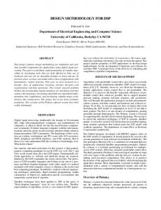
2.2.1. Fixed-Point Precision Loss and Overflow Information may be lost in fixed point operations when they produce results that have more bits than the operands [8]. For instance, the result of fixed point multiplication could potentially have as many bits as the sum of the number of bits in the two operands. In order to fit the result into the same number of bits as the operands, the answer must be rounded or truncated [9]. If this is the case, the choice of which bits to keep is very important. For instance when multiplying two fixed point numbers with the same format, with I integer bits, and F fractional bits, the answer could have up to 2*I integer bits, and 2*F fractional bits [9]. Most fixed-point multiplication procedures use the same result format as the operands. This has the effect of keeping the middle bits; the I least significant integer bits, and the F most significant fractional bits. Fractional bits below this value represent a relatively minor precision loss. If any integer bits are lost, however, the value will be radically inaccurate. This is considered to be an overflow, and needs to be avoided in embedded calculations [10]-[12]. To show the effect of the number system selection on the error Figure 1 shows a simulation of an FFT spectrum of a sinusoidal signal using: o Double-precision floating-point-numbers o Single-precision floating-point-numbers o Fixed-point numbers (width = 12, fraction = 10) with no scaling o Fixed-point numbers (width = 12, fraction = 10) with scaling, where the intermediate results are shifted right as many times as needed to avoid overflow. The final answer is multiplied by 2 raised to the power of number of left shifts needed by scaling to avoid overflow. The error of the double-precision system is the least; the error of the singleprecision system is intermediate while the error of the fixed-point system is the worst. If no scaling is used with the fixed-point system, the results are totally wrong.
6
Figure 1. FFT Spectrum Calculation Using: Double Precision Floating-Point, Single Precision Floating-Point and 12-bit Fixed-Point Without and With Scaling
2.3
An Overview of the IEEE-754 Floating-Point Standard The IEEE-754 floating-point standard is the most common real numbers
representation in today’s microprocessors, including Intel-based PC's, Macintoshes, and most Unix platforms [13]. IEEE floating point numbers have three basic components: a sign, an exponent, and a significand. The significand is composed of the fraction and an implicit leading digit (explained below). The exponent base (2) is implicit and is not stored [1].
7
Table 1 shows the layout for single (32-bit) precision IEEE standard floatingpoint values. The number of bits for each field are shown (the bit position are shown in square brackets): Table 1. IEEE-754 Storage Layout [1]
Single Precision
Sign
Exponent
Fraction
1 [31]
8 [30-23]
23 [22-00]
The Sign Bit [13] The sign bit is interpreted as follows: zero denotes a positive number and one denotes a negative number. Flipping this bit changes the sign of the number. The Exponent [13] The exponent is the component of a binary floating-point number that signifies the integer power to which two is raised in determining the value of the represented number. The Significand [13] The significand also known as the mantissa, represents the precision bits of the number. In the IEEE standard [1], it is composed of an implicit leading integer one, an implicit radix point and the fraction bits. Ranges of Floating-Point Numbers [1] The range of single precision IEEE floating point numbers is
±2 −126 to
± (2 − 2−23 ) × 2127 which is approximately equal to ±10−38 to ±3 ×1038 . Special Values [13]
The IEEE standard reserves exponent field values of all zeros and all ones to denote special values in the floating-point scheme.
8
Zero [13]
Zero is not directly representable in the normal format, due to the assumption of a leading one (it is necessary to specify a true zero significand to yield a value of zero). Zero is a special value denoted with an exponent field of all zeros and a fraction of zero. Note that -0 and +0 are distinct values, though they both compare as equal. Infinity [13]
The values +infinity and -infinity are denoted with an exponent of all ones and a fraction of zero. The sign bit distinguishes between negative infinity and positive infinity. Being able to denote infinity as a specific value is useful because it allows operations to continue past overflow situations. Operations with infinite values are well defined in IEEE floating point standard. Not a Number [13]
The value NaN (Not a Number) is used to represent a value that does not represent a real number. NaN's are represented by an exponent of all ones and a non-zero fraction. Denormalized [13]
If the exponent is all zeros, but the fraction is non zero then the value is denormalized. The units designed in this research do not support denormalized numbers.
2.4
An Overview of the Floating-Point Fused Multiply-Add (FMA) Operation [14] In 1990, IBM introduced the floating-point fused multiply-add operation on the
RISC System 6000 (IBM RS/6000) chip [3], [4]. IBM recognized that several advanced applications, specifically those with dot products, are routinely performed with a floatingpoint multiplication, A x B, immediately followed by a floating-point addition, (A x B) result + C, ad infinitum. To increase the performance of these applications, a new unit was created that merged a discrete floating-point multiplier and floating-point adder into
9
a single hardware block—the floating-point fused multiply-add unit. This floating-point arithmetic unit, shown in Figure 2, executes the equation (A x B) + C in a single instruction.
Figure 2. Block Diagram of a Floating-point Fused Multiply-add Unit, reduced from [14]
With the continued demand for 3D graphics, multimedia applications, and new advanced processing algorithms, the IEEE has included the fused multiply-add operation into the 754-2008 standard [2]. Even though the fused multiply-add architecture has troublesome latencies, high power consumption, and a performance degradation with single-instruction execution, more and more microprocessor designs implement floatingpoint fused multiply-add units in their silicon [4]-[5].
2.5
Other Fused Arithmetic Units For floating-point applications apart from the FMA, no publications or patents
were found which use fusing. There are many patents which merge multiple fixed-point arithmetic functions to speed up or reduce the area and power consumption, but since this research is concerned with floating-point, these are not relevant.
10
2.6
The Fast Fourier Transform (FFT) Algorithm Fourier analysis is a family of mathematical techniques, based on decomposing
signals into sinusoids. The Discrete Fourier Transform (DFT) is used with digitized signals [15]. The DFT of a sequence of N complex numbers is given by: N −1
X k = ∑ xn e
2π i kn N
, k = 0,..., N − 1
(1)
n =0
The Discrete Fourier Transform (DFT), can be calculated in many ways, such as solving simultaneous linear equations or correlation. The Fast Fourier Transform (FFT) is an efficient method for calculating the DFT. While it produces the same result as the other approaches, it often reduces the computation time by a factor of ten or more for large sequences [15]. There are two flavors of the FFT algorithm; decimation in time (DIT) where the time domain sequence is split into even and odd parts for processing, or decimation in frequency (DIF) where the frequency components are divided into even and odd parts for processing. The DIF and DIT are both equivalent algorithms and it is straight forward to convert from one to the other. Both the DIT and DIF can accept inputs either in order or in bit reversed order to produce bit reversed or in order outputs, respectively. Figure 3 shows the radix-2 DIT FFT and DIF FFT butterflies, which are the basic computation element in performing the FFT. Figure 4 shows the data flow diagram for performing a radix-2 DIT FFT, while Figure 5 shows the data flow diagram for performing a radix-2 DIF FFT. The X0 - X8 are the input data samples, W Nk are the twiddle factors for butterflies which is given by equation:
⎛ 2π k ⎞ ⎛ 2π k ⎞ WNk = e − i 2π k / N = cos ⎜ ⎟ − i sin ⎜ ⎟ ⎝ N ⎠ ⎝ N ⎠
11
(2)
Figure 3. Radix-2 Butterflies
Y0 Y1 Y2 Y3 Y4 Y5 Y6 Y7
X0 X4 X2
X6 X1 X5 X3 X7 Figure 4. 8-point Radix-2 DIT FFT
X0 X1
Y0 Y4 Y2 Y6 Y1
X2 X3 X4
X5 X6
Y5 Y3 Y7
X7 Figure 5. 8-point Radix-2 DIF FFT
12
2.7
Summary
In this chapter, the necessary background material needed to understand the remaining chapters was briefly covered, including a quick introduction to fixedpoint and floating point number systems. introduced as well.
13
The fast Fourier transform was
Chapter 3
Research Approach and Design Methodology
This chapter presents the research approach and the overall design flow and methodology. The general approach of performing the research is presented, then the design and implementation flow. The tools that were used are also described.
3.1
Research Approach The goal of this research is to investigate the application of fused floating-point
arithmetic for speeding up digital signal processing algorithms. Figure 6 shows the general steps taken for performing this research work. The process is summarized as: 1. Study literature about IEEE floating-point arithmetic concepts, architectures, and implementations. 2. Study literature about fused multiply-add arithmetic unit concepts, architectures and implementations. 3. Create the architecture for the fused add-subtract and fused dot-product units. 4. Prove the concept by modeling the primitive units (FPA, FPM, fused DP and fused AS) in Matlab high-level language. 5. Design the primitive units (FPA, FPM, fused DP and fused AS) in Verilog RTL language. 6. Verify the units using System Verilog testbenches and employing random stimulus generation techniques to cover a wide input range. 7. Implement the units using ASIC standard cells implementation flows where the units are mapped to a standard-cell library using synthesis, placement and routing tools. 8. Perform timing analysis on the implementations using a static timing analysis tool with extracted parasitics data from the laid-out designs.
14
Figure 6. Research Flow
15
9. Perform power consumption estimation at the gate level using the extracted parasitics from the laid-out designs. 10. Utilize primitive units RTL models (from step 5) to build RTL models for the following units: o Serial Add-Subtract (serial AS) Unit o Parallel Add-Subtract (parallel AS) Unit o Serial Dot-Product (serial DP) Unit o Parallel Dot-Product (parallel DP) Unit o Discrete Radix-2 FFT Butterfly (discrete radix-2 BF) unit o Discrete Radix-4 FFT Butterfly (discrete radix-4 BF) unit o Fused Radix-2 FFT Butterfly (fused radix-2 BF) unit o Fused Radix-4 FFT Butterfly (fused radix-4 BF) unit
11. Repeat steps 6 to 9 for all the derived units listed in step 10.
3.2
High-Level Modeling The primitive units (FPA, FPM, fused DP and fused AS), and the derived units
(serial AS, parallel AS, serial DP, parallel DP, discrete radix-2 BF, discrete radix-4 BF, fused radix-2 BF, and fused discrete radix-4 BF) architectural concepts were initially verified by modeling the functionality using the Matlab high level modeling language. High-level modeling has many merits: •
It is a fast way to verify the functionality of the new concept.
•
It is easy and fast to evaluate different architectures and fine tuning of specific architecture design options.
•
A high-level model is used as an abstract model of the design to generate input stimulus and expected results.
16
3.3
RTL Digital Design Using Verilog HDL The primitive units (FPA, FPM, fused DP and fused AS), and the derived units
(serial AS, parallel AS, serial DP, parallel DP, discrete radix-2 BF, discrete radix-4 BF, fused radix-2 BF, and fused discrete radix-4 BF) were designed from scratch using Verilog hardware description language (Verilog HDL). The functionality of the HDL designs was verified using simulation and was mapped into a technology-specific gate level implementation using synthesis. The Verilog language is one of the IEEE standardized and widely used HDL languages [16]-[18]. Verilog HDL can be used to model the system at abstract level where the functionality is modeled using high-level constructs or at the register transfer level (RTL) where the register boundaries are explicitly defined including the combinational logic enclosed by them or at the structural-level where the connection between logic gates (primitives) is described.
The RTL level (used to model the
primitive units and the derived units) is best for describing the micro-architecture and controlling the implementation details for a synthesize flow. Figure 7 shows an example Verilog model for a 2:1 multiplexer using Verilog HDL structural and RTL descriptions.
17
Figure 7. Verilog HDL for a 2:1 Multiplexer
3.4
The EDA Tools Used in The ASIC Implementation Flow To implement the primitive units (FPA, FPM, fused DP and fused AS), and all of
the derived units (serial AS, parallel AS, serial DP, parallel DP, discrete radix-2 BF, discrete radix-4 BF, fused radix-2 BF, and fused discrete radix-4 BF) the following electronic design aiding (EDA) tools were used: MathWorks Matlab [36]: Matlab is a high-level modeling tool, and a
programming language. It enables fast modeling of complex algorithms in an easy high level language. Matlab was used to verify the concepts and to build abstract models for
18
the primitive units and the derived units designs. Also it was used to generate the reference output for the error analysis experiments. Synopsys VCS Simulator [37]: Synopsys VCS is an RTL functional simulator
that can simulate Verilog, VHDL, and System C models. It has advanced capabilities that aid in the verification and test coverage of the simulated designs. It was used to verify the functionality of the primitive units and the derived units RTL models. Synopsys Design Compiler Ultra (DC Ultra) [37]: Synopsys DC Ultra is a
hardware synthesis tool. It maps an RTL hardware description model using a standard cell library into a gate-level netlist that describes the design at the structural (connectivity) level. The output design is composed of cells that exist in the standard-cell library. The synthesis tool output generation is controlled by area, delay and power constraints. DC ultra was used to map the RTL models of the primitive units, and the derived units to gate-level netlists based on the standard-cells that are available in the technology libraries. Synopsys Integrated Circuit Compiler (ICC) [37]: Synopsys IC Compiler is a
physical implementation tool that takes a gate-level netlist, a floorplan and the standardcell library as inputs, and generates a placed-and-routed design. It includes floorplanning, placement, clock tree synthesis, routing, metal fill and chip-finishing. ICC is widely adopted and recognized as the industry standard for physical implementation. The output is influenced by placement, area, power and delay constraints that control the generated design. ICC was used to place and route the primitive units and the derived units. Synopsys PrimeTime (PT) [37]: Synopsys PrimeTime is the industry standard
tool for timing sign-off. It delivers accurate timing signoff analysis that helps pinpoint timing problems prior to tapeout. A gate-level netlist, timing constraints, extracted parsitics and standard-cell libraries, are needed to sign-off the timing of the placed-androuted design. PT was used to sign-off the timing of the primitive, and the derived units. Synopsys Star-RCXT [37]: Synopsys Star-RCXT is an RLC parasitic extraction
tool. The tool inputs are the process definition file, and a physical placed-and-routed 19
design database (Synopsys Milkyway physical design database or the industry standard GDSII physical design database). Star-RCXT extracts the input design gate and wire parasitics that are necessary to perform gate-level timing analysis, and simulation based gate-level power estimation. Star-RCXT was used to extract the parasitics of the laid-out designs of the primitive units and the derived units. Synopsys PrimePower [37]: Synopsys PrimePower is a chip-level dynamic
power analysis tool. The tool inputs are a gate-level netlist, a switching activity file (SAIF) generated from the gate-level simulation, a standard-cell technology library and the extracted RC parasitics. PrimePower estimates the power consumption of the design based on the switching activity of the nets and the power-characterization data of the standard-cell library. PrimePower is integrated within Synopsys DC Ultra and ICC and can be invoked from inside these tools. PrimePower was used to estimate the power consumption of the primitive units and the derived units. Synopsys Formality [37]: Synopsys Formality checks the equivalence of two
versions of the design (i.e., RTL model versus gate-level model) to prove that they are functionally equivalent using static (non-vector based) techniques.
3.5
Functional Verification Using Simulation The correct functional behavior of the primitive units (FPA, FPM, fused DP and
fused AS) and the derived units (serial AS, parallel AS, serial DP, parallel DP, discrete radix-2 BF, discrete radix-4 BF, fused radix-2 BF, and fused radix-4 BF) was verified by comparing the simulation output of the RTL models to an abstract model that was created using System Verilog high level constructs. Figure 8 shows the flow used for performing functional verification for the primitive and the derived units. A System Verilog random stimulus generator is used to generate valid inputs that cover the full range of IEEE single-precision numbers. The stimulus is then applied to the RTL and the abstract models simultaneously and the outputs are compared. If the outputs are equal the simulation passes for the executed testcase, otherwise it fails.
20
Figure 8. Functional Verification Using Simulation
3.6
ASIC Implementation Flow At present there are three digital chip design flows in use in the industry: •
Circuit Design Flow: In this flow all of the circuits are designed at the transistor level. The functionality and timing are verified using transistor level simulation tools (SPICE). This flow typically produces the best area, speed, and the lowest power consumption. However, this flow is slow and requires large number of specialized circuit design and layout engineers. A design engineer using this flow can handle few thousand transistors (hundreds of gates) needing few months to produce the final design. At present this flow is used by the chip industry to design high-
21
density, timing and area-critical circuits such as: SRAM memories and register files and some very specialized arithmetic circuits. •
Hand placement Flow: In this flow a technology process dependent standard-cell library is used. The design RTL model is mapped to gates by design engineers and hand-placed and optimized. The functionality and timing are verified using gate-level level simulation and analysis tools. This flow typically produce good area, speed and low-power consumption. A design engineer can handle few thousands gates designs needing few months to produce the final design. However, this flow is not suitable for designs incorporating millions of gates. Moreover, this flow typically requires large teams and has a relatively slow time to market. At present, this flow is used by the chip industry to design performance-critical blocks, such as: high speed arithmetic blocks or data-path elements.
•
Automatic Synthesis, Place and Route Flow (ASIC design flow): In this flow a technology process dependent standard-cell library is used. The RTL models are mapped to gates, placed, and routed using gate-level EDA tools. The results from this flow depend on the quality and sophistication level of the EDA tools used, as well as the design constraints provided to these tools. Using typical industry-standard EDA tools result in area, delay and power consumption close to those of the hand-placement approach. This design flow produces the fastest time to market. A design engineer using this flow can “design” blocks with sizes that can go up to hundreds of thousands of gates. At present, this flow is used in the industry to design most of the chips, as long as it meets the allocated area, delay and power consumption budgets.
The ASIC design flow was used to implement the primitive units (FPA, FPM, fused DP and fused AS), and the derived units (serial AS, parallel AS, serial DP, parallel 22
DP, discrete radix-2 BF, discrete radix-4 BF, fused radix-2 BF, and fused discrete radix-4 BF). The ASIC design flow used in this research is composed of two main sub-flows: the implementation sub-flow, and the analysis sub-flow. The implementation sub-flow (shown in Figure 9) includes the following steps:
1. Synthesis: The Verilog RTL models of the primitive and the derived units are mapped into a technology specific library (described in Section 3.7) using the Synopsys Ultra DC synthesis tool. The output of this step is a gate level netlist that is used by the placement and routing tool. 2. Floorplan: The floorplan defines the design size, the pre-placement of macros, and the placement of the primary input/output ports. For a full chip design, floorplanning of any sub-block is based on the placement of the sub-block relative to other sub-blocks, and its connectivity. For the primitive and derived units designed in this dissertation, the following floorplan methodology was used: o Each unit was implemented as a standalone block that can be
used as part of a full-chip design. o The size of each unit (i.e., floorplan size) was a design
parameter. It was forced to be 135% of the area of a first pass implementation using the Synopsys ICC minimum physical constraints (MPC) mode. As a result, the overall utilization was ~75% of the total unit (floorplan) area. The remaining 25% of the floorplan area was left for routing - a reasonable value for ASIC design flows in the industry.
23
Figure 9. Implementation Sub-Flow
24
o The placement of primary inputs and outputs was automatic.
The tool was allowed to choose the initial placement using the MPC mode. In addition, after the first pass of design placement, an automatic inputs/outputs placement optimization is performed. o The inputs/outputs on the top and bottom edges of the design
were placed on metal layer three. o The inputs/outputs on the right and left sides of the design were
placed on metal layer four.
3. Placement: In this step, placement of the gate-level netlist (of the primitive and derived units) is done in the floorplan generated in step 2 using Synopsys ICC.
Synopsys ICC optimizes the placement based
on the design constraints to achieve the placement with lowest overall design area, power consumption and best timing. 4. Routing: A nine metal layers process (described in Section 3.7) was used to route the primitive and derived units. The placed designs of the primitive and derived units were routed using Synopsys ICC. The lower 6 process metal layers were used for routing, and the remaining top 3 metal layers were left to be used by chip-level power and clock routing (this is an industry standard practice for similar designs). The goal of this step is to produce a 100% connected design, with no process design rules violations (i.e., DRC clean), and to generate a layout versus schematic equivalent (i.e., LVS clean) design.
25
The analysis sub-flow (shown in Figure 10) includes the following steps:
1. RC parasitics extraction using Synopsys Star-RCXT: The base technology libraries information (described in Section 3.7), in addition to the routing of the primitive and derived designs are used by Synopsys Star-RCXT to extract wiring resistance, capacitance, and the gates input/output parasitics. 2. Static timing analysis (STA) using Synopsys PT: For all of the primitive and derived units, the gate-level netlist, the design constraints, and the extracted RC parasitics (from step 1 above) are used by synopsys PT to verify timing and performance targets. The maximum possible operating frequency is determined in this step. Also the designs are verified to be free from any setup, hold and/or other timing violations that may limit the operating frequency. 3. Power analysis using Synopsys PrimePower: The RC parasitics, the gate-level netlist, and a carfully designed stimulus are used by Synopsys PrimePower to estimate the power consumed by the primitive and the derived unit designs. The stimulus used needs to be designed carefully to make sure it represents the mainstream usage of the design, otherwise the power estimates will be skewed toward an unrealistic usage pattern (the power estimation flow is described in detail in Section 3.6.1). 4. Formal Verification using Synopsys Formality: The RTL model is compared to the final gate level netlist to verify that they are functionally equivalent.
26
FPA, FPM, Fused AS, Fused DP, Serial AS, Parallel AS, Serial DP, Parallel DP, Discrete radix-2 BF, Discrete Radix-4 BF, Fused Radix-2 BF and Fused Radix-4 BF
RC Extraction Tool (Synopsys Star-RCXT)
...0010010101… ...0011010101... ...0001010101...
A B
Static Timing Analyzer (Synopsys PT)
Power Analysis Tool (Synopsys PrimePower)
Figure 10. Analysis Sub-Flow
27
OU T
3.6.1. Dynamic Power Estimation Detailed Methodology To estimate the power consumption of the circuits of the primitive units (FPA, FPM, fused DP and fused AS), and the power consumption of the circuits of the derived units (serial AS, parallel AS, serial DP, parallel DP, discrete radix-2 BF, discrete radix-4 BF, fused radix-2 BF, and fused discrete radix-4 BF) the following methodology was used: 1. Stimulus selection: The following factors were considered to design the input stimulus : a. Input data switching rate and switching distribution over time determines the power consumption [42]. b. There is no universal model or method for selecting the input stimulus that works for different type of circuits under different usage scenarios. Many publications have proposed a statistical model for determining the appropriate switching rate for combinational and sequential circuits [42]-[43]. According to [42] for combinational designs a switching rate around 40% and switching distribution (percentage of the simulation time where the signals are changing states) around 40% is acceptable for evaluating the power consumption of combinational logic such as ALU’s and other arithmetic circuits. c. The FPA, the FPM, the fused DP and fused AS primitive units, and the parallel AS, the parallel DP, the discrete radix-2 BF, the discrete radix-4 BF, the fused radix-2 BF, and the fused discrete radix-4 BF derived units are purely combinational. The serial AS and the serial DP derived units are dominated (more than 87% is combinational) by combinational logic. As a result, in this research an input pattern was used with the input bits switching twice every
28
four cycles (50% data switching rate and 50% switching distribution) which is slightly more aggressive than the recommended range in [42]-[43]. d. This research goal is not to determine the absolute power consumption figures (determined largely by the input pattern) for the primitive and the derived units. This research is concerned with comparing the relative power consumption of the various design options of the primitive and the derived units. e. The primitive and the derived units were driven with the same input patterns which leads to accurate relative power consumption comparison because all the equivalent design units were exposed to the same input patterns. 2. Stimulus generation using Matlab: a. A large set of 100,000 random numbers that covers the full range of IEEE single precision floating-point numbers was generated. b. The “RANDC” function was used to generate these numbers which guaranties that the same number will not repeat. c. The randomly generated numbers were studied using Matlab, and each individual bit of the generated numbers changed states from 0Æ1Æ0 every 4 cycles. 3. Simulation using Synopsys VCS: a. For each of the primitive and derived design units, the gate level netlist was simulated using the stimulus generated in step 1 above. b. A value change dump file was produced from the simulation and converted to a “SAIF” file (it contains information about the toggle rate per time unit for each signal in the design, in addition to the static probability of having the signal stuck at logic one). 4. Power estimation using Synopsys PrimePower:
29
a. For each of the primitive and derived design units, the “SAIF” file generated in step 3, the gate level netlist, and the placed-and-routed design extracted parasitics were used by Synopsys PrimePower to estimate the average consumed power. b. The average power consumption was used as the design unit average power consumption value. It is reported in Chapters 4 to 6 of this dissertation.
3.7
The 45nm CMOS Technology Process Used to Implement the Primitive and the Derived Units In a semiconductor manufacturing process, many processes and dozens of steps
are needed to create an integrated circuit [38]. Some of the important characteristics of a semiconductor manufacturing process are: •
Channel-Length of the minimum size transistor that can be fabricated, the smaller the transistor size the faster, lower power and more dense chips could be produced. Technology processes are tagged by this parameter, for example a 45nm technology process is capable of fabricating transistors with a channel length of 45nm.
•
Number of Interconnect layers: The more transistors that are packed on a chip, the more interconnect layers that are needed to connect them. Modern processes use from 7-11 metal layers depending on the target application.
•
Target application: Technology processes at certain technology node have many
flavors
based
on
the
target
products.
For
high
speed
microprocessors, a high-performance process is used that is usually tuned to create the maximum possible transistor speed (usually at the expense of extra power consumption). For mobile applications, a low-leakage, and low-power process is used, the process is tuned to sacrifice speed and performance to produce lower power designs. 30
•
Bulk CMOS manufacturing technology and silicon on insulator (SOI) manufacturing technology are the industry dominant technologies for digital designs.
An industrial 45nm technology process was used in this research to deign the primitive units (FPA, FPM, fused DP and fused AS), and the derived units (serial AS, parallel AS, serial DP, parallel DP, discrete radix-2 BF, discrete radix-4 BF, fused radix-2 BF, and fused discrete radix-4 BF), The technology process that was used has the following characteristics: •
A
45nm
high-performance
industry-standard
semiconductor
manufacturing process. •
A 9-metal layer process, with the lower six metal layers used for routing the units and the top three layers reserved for the clock routing and power distribution.
•
A bulk CMOS process.
•
The standard-cells used to map the primitive and the derived units RTL models to gate-level netlists are designed for high-performance applications.
3.8
Notes About ASIC Standard-Cell Libraries and ASIC Flows Application-specific integrated circuits (ASIC) are integrated circuits designed for
a specific application. The ASIC design flow includes the design of a large set of standard-cells for a specific technology node.
This standard-cell library is designed
according to the target product and could have many flavors, such as: low-power cells with slower speed, or fast cells at the expense of higher power consumption. The standard-cells are characterized at the transistor level for power, delay, transition time and noise. The information that describes the standard-cell library (i.e.,
31
functionality, area, power, transition time, delay, etc.) is listed in databases are used by the synthesis tools to map the RTL models to the appropriate gates. A standard-cell library typically includes many logic gates: NAND gates, NOR gates, X-OR gates, inverters, multiplexers, latches, flops-flops, and much more. Many versions of the same gate (NANDx1, NANDx2, NANDx3, …etc…) are usually included based on the intended drive capability. For example, a technology-library may have eight logic NAND gates that differ in their output transistor sizes, gate area, gate delay, input and output transition time and their current drive capabilities. The quality of the standardcell library determines the quality of the synthesized design. The design area, delay and power constraints, as well as the floorplan (macro placement and input/output port locations) influence the selection of certain standardcells to implement a function. RTL design mapping is a function of the technologylibrary, floorplan, and implementation constraints. Changing the floorplan may result in a smaller (or bigger) size of the overall pure silicon gates used to realize a design due to a reduction (or increase) in number of gates, and/or wire lengths that a gate needs to drive.
32
Chapter 4
Floating-Point Fused Add-Subtract Unit
A floating-point fused add-subtract unit is presented that performs simultaneous floating-point add and subtract operations on a common pair of single-precision floatingpoint data in about the same time that it takes to perform a single addition with a conventional floating-point adder. This unit uses the IEEE-754 single-precision format and supports all rounding modes. When placed and routed in the automatic synthesis ASIC implementation design flow described in Section 3.6 and the 45nm standard cell libraries described in Section 3.7, the fused add-subtract unit is only about 56% larger than a conventional floating-point adder, and consumes 50% more power than the conventional floating-point adder.
4.1
Introduction This chapter introduces the floating-point fused add-subtract unit. The design and
implementation results using the automatic synthesis ASIC implementation design flow described in Section 3.6 and the industry standard 45nm process described in Section 3.7 are presented. In many DSP algorithms both the sum and difference of a pair of operands are needed for subsequent processing. This is required, for example, in computation of the FFT butterfly operation. In traditional floating-point hardware these operations may be performed in a serial fashion which limits the throughput. The use of a fused add-subtract (fused AS) unit accelerates the butterfly operation. Alternatively, the addition and subtraction may be performed in parallel with two floating-point adders which is expensive (in silicon area and in power consumption). This chapter presents the implementation of the floating-point fused add-subtract unit shown in Figure 11. The fused add-subtract unit performs the following operations:
33
x
=
a
+
b
y
=
a
−
b (3)
Figure 11. The Floating-Point Fused Add-Subtract Unit Concept
4.2
Floating-Point Adder Design The most frequent floating-point operations are addition and subtraction, and
together they account for 55% of the total floating-point operations in typical scientific applications [22]. Both addition and subtraction use the floating-point adder. Techniques to reduce the latency and increase the throughput of the floating-point adder have therefore been the subject of much previous research [23]-[28]. Due to its many inherently serial component operations, floating-point addition can have a longer latency than floating-point multiplication. Pipelining is a commonly used method to increase the throughput of the adder, but it does not reduce the latency. Previous research has provided algorithms to reduce the latency by performing some of the operations in parallel. This parallelism is achieved at the cost of additional hardware. The minimum achievable latency using such algorithms in high clock-rate microprocessors has been three cycles, with a throughput of one add per cycle.
4.2.1. Basic Floating-Point Addition Algorithm The straightforward basic floating-point addition algorithm requires the most serial operations. It has the following steps [22]:
34
1. Exponent subtraction: Perform subtraction of the exponents to form the absolute difference Ea − Eb = d . 2. Alignment: Right shift the significand of the smaller operand by d bits. The larger exponent is denoted E f . 3. Significand addition: Perform addition or subtraction according to the effective operation. The result is a function of the op-code and the signs of the operands. 4. Conversion: Convert a negative significand result to a sign-magnitude representation. The conversion requires a two's complement operation, including an addition step. 5. Leading-one detection: Determine the amount of left shift needed in the case of subtraction yielding cancellation. For addition, determine whether or not a 1-bit right shift is required. Then priority-encode the result to drive the normalizing shifter. 6. Normalization: Normalize the significand and update E f appropriately. 7. Rounding: Round the final result by conditionally adding 1-ulp as required by the IEEE standard. If rounding causes an overflow, perform a 1-bit right shift and increment E f . The latency of this algorithm is large, due to its many long length components. The steps describing the latency of this algorithm are listed in Table 2. Figure 12 shows the block diagram of an architecture that realizes this algorithm.
35
Table 2. Basic Floating-Point Adder Algorithm Latency Step
1 2
Operation
Latency
Step Dependency
Exponent subtraction Right shift smaller operand significand Significand addition
1 Exponent subtract delay 1 Significand full-length shift delay
None Step 1
1 Full-length significand addition delay
Step 2
Sign-magnitude conversion Leading-one detection Normalization
1 Full-length significand addition delay
Step 3
Rounding
1 Full-length significand addition delay Steps 1, 5 and + 1-bit right shift 6
3 4 5
1 Leading-one detection delay 1 Full-length shift operation delay
Step 4 Steps 1 and 4
6 7
36
Figure 12. A Conventional Floating-Point Adder
4.3
Fused Add-Subtract Unit Design Approachs There are two design approaches that can be taken with discrete floating-point
adders to realize the add-subtract function. These are the parallel implementation shown in Figure 13 where two adders operate in parallel (one adding and one subtracting) and the serial implementation shown in Figure 14 where a single adder is used twice (once adding and once subtracting) with the same operands.
37
a
a+b
b a −b
Figure 13. Conventional Parallel Realization of an Add-Subtract Unit
a
a + b
b
a−b
Figure 14. Conventional Serial Realization of an Add-Subtract Unit
In a parallel conventional implementation of the fused add-subtract (such as that shown in Figure 13) two floating-point adders are used to perform the operation. This approach is fast, however, the area and power overhead is large because two floatingpoint add/subtract units are used. In a serial conventional implementation of the fused add-subtract (such as that shown in Figure 14) one floating-point adder/subtracter is used to perform the operation in addition to a storage element to store the addition or subtraction result. This approach is very efficient in terms of area. However, due to the serial execution of both operations, the time needed to get both results is twice the time needed by the parallel approach. Also since a storage element is used, it adds slightly to the area and power overhead.
38
Moreover, power is consumed for a longer time due to executing the add/sub operation twice. The architecture of the fused add-subtract unit is derived from the floating-point add unit. The exponent difference, significand shift and exponent adjustment functions can be performed once with a single set of hardware, with the results shared by both the add and the subtract operations. New add and normalize blocks are needed for the new subtract operation. Figure 15 shows the architecture of the fused add-subtract unit, the blocks with white background are the same blocks used for a single floating-point add operation. The blocks with green background are additional blocks used to perform the subtract operation, and the blocks with yellow background are similar to the floatingpoint add blocks, but with extended functionality to calculate the sign and exponent for the new subtract operation.
Figure 15. Floating-Point Fused Add-Subtract Unit
39
4.4
Implementation Results To study the merits of the fused add-subtract unit, the following units were
designed: •
Basic Floating-Point Adder (FPA)
•
Serial Floating-Point Add-Subtract Unit (serial AS)
•
Parallel Floating-Point Add-Subtract Unit (parallel AS)
•
Floating-Point Fused Add-Subtract Unit (fused AS)
This section presents the implementation results of the above units using the implementation flow described in Chapter 3.
4.4.1. Floating-Point Adder (FPA) Unit The basic floating-point adder (FPA) was designed using the architecture of the adder shown previously in Figure 12. The basic floating-point adder is composed of the following main sub-circuits: Align Circuit: This circuit (shown in Figure 16) detects the difference between
the exponents of the two operands and aligns the significands of the two operands for addition or subtraction by shifting the smaller significand by an amount proportional to the difference between the exponents of the two operands.
40
A
B Significand B Significand A
Compare the Exponents
MUX2:1
Shift Amount
Larger Exponent
Shifter
Smaller Operand Aligned Significand
Shift Amount
MUX2:1
Larger Operand Significand
Figure 16. Align Circuit
Significand Add/Subtract Circuit: This circuit (shown in Figure 17) performs
the addition or subtraction operation of the significands. It detects the effective operation based on the signs of the two operands and the intended operation. It also generates guard and presticky bits that aid in the proper rounding of the final results.
41
Figure 17. Significand Adder Circuit
Normalization Circuit: This circuit (shown in Figure 18) detects the number of
leading zeros in the significand adder result, and left-shifts the sum to have a leading one in the left-most digit for IEEE floating-number format compliance. It also generates exponent correction value, as well as round and sticky bits that are used by the rounding circuit.
Figure 18. Normalization Circuit
42
Rounding Circuit: This circuit (shown in Figure 19) rounds the final result
according to the selected IEEE rounding mode.
Figure 19. Rounding Circuit
Finalization Circuit: This circuit (shown in Figure 20) assembles the final sign,
exponent and final significand to generate the results. Also, it generates overflow, zero and other special flags required by IEEE compliant adders.
Figure 20. Finalization Circuit
43
4.4.1.1. Timing The FPA was implemented using the automatic synthesis ASIC implementation design flow described in Section 3.6 and the 45nm standard cell libraries described in Section 3.7. The placed-and-routed FPA computes a floating-point addition in 1.64ns. The critical timing path of the FPA is detailed in Table 3.
Table 3. Floating-Point Adder Critical Timing Path Sub-Circuit
Latency (ns)
Input External Delay
0.1
Allign
0.4
Significand Adder
0.2
Normalizer
0.4
Rounder
0.2
Assembler
0.2
Output External Delay
0.1
Total
1.64
4.4.1.2. Place and Route Results Figure 21 shows the placed-and-routed FPA. The FPA occupies an area of 72μm by 72μm with 75% utilization for gates/circuits, and the remaining 25% for routing.
44
Figure 21. Floating-Point Adder Unit Routing
Figure 22 shows the FPA placement. The major FPA sub-circuits are colored differently and the critical timing path is highlighted.
45
Figure 22. Floating-Point Adder Unit Placement with the Critical Timing Path Highlighted
The pure gates area of the FPA is 3,811μm2. Table 4 lists the area distribution of the main FPA sub-circuits.
46
Table 4. Floating-Point Adder Area Distribution Unit
Area (μm2)
%
Align
1,404
36.8
Significand Adder
738
19.4
Normalizer
989
26
Rounder
317
8.3
Assembler
321
8.4
Special Case Detection
42
1.1
3,811
100
Total
4.4.1.3. Power and Energy Estimation Results Table 5 lists the power consumption of the FPA sub-circuits using the power estimation methodology described in Section 3.6.1. Table 5. Floating-Point Adder Total Power Distribution Unit
Average Power (mW)
%
Align
2.53
37.9
Significand Adder
1.76
26.4
Normalizer
1.52
22.8
Rounder
0.47
7.1
Assembler
0.43
6.5
Special Case Detection
0.04
0.7
Total
6.76
100.00
The energy consumption of the FPA unit can be calculated by multiplying the delay of the FPA unit by its power consumption which results in 11.5 pJ.
4.4.2. Serial Add-Subtract (Serial AS) Unit Figure 23 shows the micro-architecture of the serial add-subtract unit (serial AS). One adder/subtracter is used to perform the addition and subtraction operations in serial fashion. Serial add and subtract operations need at least two clock cycles. A finite state machine controls the operation of the serial AS unit.
47
a
a + b
a −b
b
Figure 23. Serial AS Micro-Architecture
4.4.2.1. Timing The serial AS was implemented using the automatic synthesis ASIC implementation design flow described in Section 3.6 and the 45nm standard cell libraries described in Section 3.7. The placed-and-routed design computes a floating-point addition or subtraction in 1.7ns. The critical timing path of the serial AS is detailed in Table 6. To generate the addition and the subtraction results of the two operands, two clock cycles are needed totaling 3.42ns.
48
Table 6. Serial AS Critical Timing Path Sub-Circuit
Latency (ns)
Input External Delay
0.1
Adder
1.4
Register Loading
0.1
Output External Delay
0.1
Total
1.7
4.4.2.2. Place and Route Results Figure 24 shows the placed-and-routed serial AS unit. The serial AS occupies an area of 77μm by 77μm with 75% utilization for gates/circuits and the remaining 25% for routing.
49
Figure 24. Serial AS Unit Routing
Figure 25 shows the serial AS placement. The major serial AS sub-circuits are colored differently and the critical timing path is highlighted.
50
Figure 25. Serial AS Unit Placement with Critical Path Highlighted
The pure gates area of the serial AS is 4,344μm2. Table 7 lists the area distribution of the serial AS main sub-circuits.
51
Table 7. Serial AS Area Distribution Unit Adder Add Result Register Subtract Result Register
Area (μm2) 3,740 302 302
% 86 7 7
4,344
100
Total
4.4.2.3. Power and Energy Estimation Results Table 8 lists the power consumption of the serial AS sub-circuits using the power estimation methodology described in Section 3.6.1. Table 8. Serial AS Average Power Distribution Unit
Power (mW)
%
Adder
6.26
91.2
Add Result Register
0.30
4.4
Subtract Result Register
0.30
4.4
Total
6.86
100
The energy consumption of the serial AS unit can be calculated by multiplying the delay of the serial AS unit by its power consumption which results in 24.3 pJ.
4.4.3. Parallel Add-Subtract (Parallel AS) Unit The parallel AS unit was implemented using the architecture shown previously in Figure 13. Two floating-point adders operating in parallel are used to realize the simultaneous add/subtract function.
4.4.3.1. Timing The parallel AS unit was implemented using the automatic synthesis ASIC implementation design flow described in Section 3.6 and the 45nm standard cell libraries described in Section 3.7. The placed-and-routed design computes a simultaneous
52
floating-point addition and subtraction in 1.7ns. The critical timing path of the parallel AS is detailed in Table 9. Table 9. Parallel AS Critical Timing Path Sub-Circuit
Latency (ns)
Input External Delay
0.1
Adder/Subtracter
1.5
Output External Delay
0.1
Total
1.7
4.4.3.2. Place and Route Results Figure 24 shows the placed-and-routed parallel AS unit. The parallel AS unit occupies an area of 100μm by 100μm with 75% utilization for gates/circuits and the remaining 25% for routing.
53
Figure 26. Parallel AS Unit Routing
Figure 27 shows the parallel AS placement. The major parallel AS sub-circuits are colored differently and the critical timing path is highlighted.
54
Figure 27. Parallel AS Unit Placement with Critical Timing Path Highlighted
The pure gates area of the parallel AS is 7,456 μm2. Table 10 lists the area distribution of the parallel AS main sub-circuits.
Table 10. Parallel AS Area Distribution Area (μm2)
%
Adder
3,787
50.8
Subtracter
3,664
49.1
Total
7,456
100
Unit
55
4.4.3.3. Power and Energy Estimation Results Table 11 lists the power consumption of the parallel AS sub-circuits using the power estimation methodology described in Section 3.6.1.
Table 11. Parallel AS Total Power Distribution Unit
Average Power (mW)
%
adder
6.41
50
subtracter
6.40
50
Total
12.83
100.00
The energy consumption of the parallel AS unit can be calculated by multiplying the delay of the parallel AS unit by its power consumption which results in 22.2 pJ.
4.4.4. Fused Add-Subtract (Fused AS) Unit The fused AS unit was implemented using the architecture shown previously in Figure 15. This design starts from the basic FPA architecture shown previously in Figure 12. Since the same two operands are being added and subtracted, the exponent circuit can be shared between the add and subtract sub-functions. Two units are duplicated: the significands adder to perform the simultaneous significand subtract, as well as the rounding and the normalization circuits necessary to round and normalize the significand subtract result. The rest of the fused AS sub-circuits’ functionality are exactly the same as the FPA equivalent sub-circuits.
4.4.4.1. Timing The fused AS unit was implemented using the automatic synthesis ASIC implementation design flow described in Section 3.6 and the 45nm standard cell libraries described in Section 3.7. The placed-and-routed design computes a simultaneous
56
floating-point addition and subtraction in 1.72ns. The critical timing path of the fused AS is detailed in Table 12.
Table 12. Fused AS Critical Timing Path Sub-Circuit
Latency (ns)
Input External Delay
0.1
Aligner
0.3
Significand Add/Subtract
0.3
Normalizer
0.4
Rounder
0.3
Assembler
0.2
Output External Delay
0.1
Total
1.72
4.4.4.2. Place and Route Results Figure 28 shows the placed-and-routed fused AS unit.
The fused AS unit
occupies an area of 90μm by 90μm with 75% utilization for gates/circuits and the remaining 25% for routing.
57
Figure 28. Fused AS Unit Routing
Figure 29 shows the fused AS placement. The major fused AS sub-circuits are colored differently and the critical timing path is highlighted.
58
Figure 29. Fused AS Unit Placement with Critical Timing Path Highlighted
The fused AS pure gates area is 5,947μm2. Table 13 lists the area distribution of the main fused AS sub-circuits.
59
Table 13. Fused AS Area Distribution Area (μm2)
%
Aligner
1,482
24.9
Significand Add/Subtract
1,138
19.1
Adder Normalizer
988
16.6
Subtracter Normalizer
936
15.7
Add/Subtract Rounder
643
10.8
Special Case Detection
42
0.7
Assembler
713
12
Miscellaneous
4.6
0.08
5,947
100
Unit
Total
4.4.4.3. Power and Energy Estimation Results Table 14 lists the power consumption of the fused AS sub-circuits using the power estimation methodology described in Section 3.6.1. Table 14. Fused AS Average Power Distribution Unit
Average Power (mW)
%
Aligner
2.74
27
Significand Add/Subtract
2.43
23.9
Adder Normalizer
1.60
15.8
Subtracter Normalizer
1.45
14.3
Add/Subtract Rounder
0.96
9.4
Special Case Detection
0.046
0.4
Assembler
0.92
9.1
Miscellaneous
0.006
0.054
Total
10.15
100
The energy consumption of the fused AS unit can be calculated by multiplying the delay of the fused AS unit by its power consumption which results in 17.2 pJ.
60
4.5
Add-Subtract Unit Implementation Results Summary This chapter presents the implementation results of a floating-point fused add-
subtract (fused AS) unit in addition to the implementation results of a floating-point adder, a serial AS, and a parallel AS. The following tables and figures summarize the implementation results for the units presented in this chapter by using the floating-point adder’s delay, area, power, and energy numbers as the reference. Table 15. Add-Subtract Unit Delay Comparison for Performing Simultaneous Add and Subtract on Two Operands Unit
Delay (ns)
% of FPA
FPA
1.64
100
Serial AS
3.42
208
Fused AS
1.72
105
Parallel AS
1.70
104
250
200
150 % of FPA 100
50
0 % of FPA
FPA
Serial AS
Fused AS
Parallel AS
100
208
105
104
Figure 30. Add-Subtract Unit Delay Comparison
61
Table 16. Add-Subtract Unit Area Comparison Unit
Area (μm2)
% of FPA
FPA
3,811
100
Serial AS
4,344
114
Fused AS
5,947
156
Parallel AS
7,456
196
250
200
150 % of FPA 100
50
0 % of FPA
FPA
Serial AS
Fused AS
Parallel AS
100
114
156
196
Figure 31. Add-Subtract Unit Area Comparison
62
Table 17. Add-Subtract Unit Power Consumption Comparison Unit
Average Power (mW)
% of FPA
FPA
6.76
100
Serial AS
6.86
102
Fused AS
10.15
150
Parallel AS
12.83
190
200 180 160 140 120 100
% of FPA
80 60 40 20 0 % of FPA
FPA
Serial AS
Fused AS
Parallel AS
100
102
150
190
Figure 32. Add-Subtract Unit Power Consumption Comparison
63
Table 18. Add-Subtract Unit Energy Consumption Comparison Unit FPA Serial AS Fused AS Parallel AS
Energy (pJ) 11.5 24.3 17.2 22.2
% of FPA 100 208 150 193
250
200
150 % of FPA 100
50
0 % of FPA
FPA
Serial AS
Fused AS
Parallel AS
100
208
150
193
Figure 33. Add-Subtract Unit Energy Consumption Comparison
The fused AS unit achieves the performance level of a parallel AS while showing a significant savings in area.
The area overhead of the fused AS over the serial AS is
32%. The power consumption of the fused AS unit is midway between the serial and the parallel approaches, with 48% overhead over the serial approach. The energy consumed by the fused AS unit is 30% less than the serial approach and 22% less than the energy consumed by the parallel approach which makes the fused AS unit more attractive for battery operated devices. The fused AS unit has been introduced, and the implementation results (using a bulk-CMOS mobile SOC 45nm process) were published in [33]. 64
Chapter 5
Floating-Point Fused Two-Term DotProduct Unit
This chapter presents a floating-point fused two-term dot-product unit. This unit performs single-precision floating-point multiplication and addition operations on two pairs of data in a period of time that is only 150% greater than that required for a single conventional floating-point multiplication. This unit uses the IEEE-754 single-precision format and supports all rounding modes. When placed-and-routed in a 45nm process (described in Section 3.7), the fused dot-product unit occupies about 70% of the area needed to implement a parallel dot-product unit using conventional floating-point adders and multipliers implemented with the same process. The speed of the fused dot-product is about 27% faster than the conventional parallel approach. The numerical result of the fused unit is more accurate because only one rounding operation is used, versus three for the conventional approach.
5.1
Introduction Similar to the operations performed by the fused multiply-add unit, in many DSP
algorithms, calculating the sum of the products of two sets of operands (i.e., a two-term dot-product) is a frequently used operation. For example, this is required in the computation of the FFT and DCT butterfly operations. In a traditional implementation, the dot-product is performed with two multiplications and an addition. These operations may be performed in a serial fashion (as shown in Figure 34) by utilizing a single adder and a single multiplier with multiplexers and registers for intermediate results. It has low throughput, has a small area and low power consumption. Alternatively, the multiplications may be performed in parallel with two independent multipliers followed by an adder (as shown in Figure 35). This alternative (parallel approach) is expensive (in silicon area and in power
65
consumption). It is, however, appropriate for applications where maximizing the throughput is more important than minimizing the area or the power consumption.
Figure 34. Two-Term Dot-Product Serial Implementation
Figure 35. Two-Term Dot-Product Parallel Implementation
This chapter introduces a floating-point fused two-term dot-product (fused DP) unit. The floating-point fused two-term dot-product unit shown in Figure 36 performs the following operation: y = (a × b ± c × d )
(4)
66
Figure 36. The Fused DP Unit Concept
The numerical operation performed by this unit can be used to improve many DSP algorithms. Specifically, multiplication of complex numbers benefits greatly from the fused DP unit as shown in the following equation: Y = yre + jyim = ( are + jaim ) × (bre + jbim ) = ( arebre − aimbim ) + j ( arebim + bre aim )
(5)
In an implementation with discrete floating-point adders and multipliers six operations are required (two adders and four multipliers) as shown in Figure 37. Alternatively two fused two-term dot-product units can be used: the three elements with green background are realized with one fused two-term dot-product unit, and the three elements with blue background are realized with a second fused two-term dot-product unit.
67
b re a re y re
a im b im b im
a re y im
a im b re Figure 37. Complex Multiplier Computation
5.2
Floating-Point Multiplier Design The largest logical block in a floating-point unit is the floating-point multiplier. It
usually takes two input operands and provides a multiplied and rounded result. The unit itself, when compared to a floating-point adder, has a simpler overall architecture, but contains complex components that occupy large area and use many routing resources [29]. The floating-point multiplier by itself has fast performance with low latency; however, many designs add an array of complex arithmetic functions beyond simple multiplication to the floating-point multiplier in order to process transcendental, divide, and square root algorithms that use ROM tables and to perform multiplicative iterations. Also, if the multiplier is designed to accept a denormal input then the area and delay will be increased substantially. For this research a basic floating-point multiplier is used.
68
5.2.1. Basic Floating-Point Multiplier Algorithm Floating point multiplication consists of an exclusive-OR of the signs, an addition of the exponents and a multiplication of the significands. The significand multiplication is an unsigned fixed-point multiplication. The most appropriate multipliers for the significand multiplication are the tree multipliers [30], due to their high performance. The typical structure of a tree multiplier [30] consists of: 1. Formation of the binary bit products with an array of AND gates. 2. A partial product reduction tree. This can be either a Wallace tree or Dadda reduction that reduces the bit products to two words. 3. A final carry propagate adder, that sums the two words to generate the product. If the input numbers have m-bit sizes, then the final propagate adder has a bit less than 2•m-bit size.
However, because of operating with IEEE 754 floating point numbers, several challenges appear [31]: 1.
The significands are numbers in the [1,2) interval. Consequently, the result
is a number in the [1,4) interval. Therefore, a normalization step (a one position rightshift of the significand, followed by an increment of the exponent) may be needed. 2.
After the significand multiplication, a double-size significand will result.
Thus, a rounding step is needed. This rounding step may require a plus-one addition to the significand of the result. Therefore a large carry propagate adder is required.
Several methods for latency reduction in the rounding step have been developed, such as the ES algorithm, the YZ algorithm and the QTF algorithm [31]. The basic floating-point multiplier architecture is shown in Figure 38.The unit begins processing data in a radix-8 Booth encoded multiplication tree. The multiplier tree result passes to a combined add/round stage, where the carry/save product is combined and rounded. The round and post normalize stage outputs the rounded result and the
69
floating-point multiplication is complete. Both the sign and the exponent datapaths run in parallel to the significand processing.
Figure 38. Basic Floating-Point Multiplier
70
5.3
Fused DP Unit Design Approach The floating-point fused two-term dot-product unit architecture is derived from
the architecture of a floating-point fused multiplier-adder. A conventional single path floating-point fused multiplier-adder architecture is shown in Figure 39 [14]. An exponent compare circuit, a second multiplier reduction tree, and a 4:2 CSA adder are added to convert the fused multiplier-adder into the fused two-term dot-product unit shown in Figure 40. The fused DP unit can perform either the addition or subtraction of the products by complementing the outputs of one of multiplier trees for subtraction. The exponent compare circuit for the floating-point fused two-term dot-product unit is based on the exponent compare circuit for the FMA that is shown in Figure 41. The fused DP exponent compare circuit shown in Figure 42 has an extra exponent adder (an 8-bit adder for single-precision IEEE floating-point) to add the exponents of inputs C and D. The fused DP unit extra exponent adder is working in parallel with the FMA unit original exponent adder so the delay of the fused DP unit exponent compare circuit will be almost equal to the delay of the FMA exponent compare circuit. The leading zero anticipator (LZA) circuit concept is shown in Figure 43. It is composed of a pre-encoder and a leading zero detector [39]-[40]. The LZA circuit is necessary for normalization of the result especially for fused DP unit subtraction operations with massive cancellation (the result includes many leading zeros). The normalize and the round blocks of the fused DP unit are similar to the FPA unit normalization and rounding circuits (shown previously in Figures 19 and 20, respectively). The alignment circuit of the floating-point fused two-term dot-product unit is based on the alignment circuit of the FMA unit. The fused DP alignment circuit shown in Figure 44 has two wide alignment shifter sub-blocks. This provides the sum and carry outputs of the “C*D” significand multiplication result. The sum and carry outputs of “C*D” significand multiplication are aligned to the outputs of “A*B” significand multiplication according to the relative magnitude of “A*B” versus “C*D” as shown in Figure 44. 71
Figure 39. Conventional Floating-Point FMA unit [14]
72
Figure 40. Floating-Point Fused Two-Term Dot-Product Unit
73
Figure 41. Floating-Point Fused Multiply-Add Unit Exponent Compare Circuit
74
Figure 42. Floating-Point Fused Two-Term Dot-Product Unit Exponent Compare Circuit
y(n) 1 0 0 0 …
y(n-1) x 1 0 0 …
y(n-2) x x 1 0 …
y(n-3) x x x 1 …
Figure 43. LZA Circuit Concept [39]
75
… x x x x …
y(0) x x x x …
Shift Count 0 1 2 3 …
Figure 44. Floating-Point Fused Two-Term Dot-Product Unit Alignment Circuit
5.4
Dot-Product Unit Implementation Results To show the merits of the floating-point two-term fused dot-product unit, the
following units were designed: •
Basic Floating-Point Multiplier (FPM) Unit
•
Serial Floating-Point Dot-Product (serial DP) Unit
•
Parallel Floating-Point Dot-Product (parallel DP) Unit
•
Fused Floating-Point Dot-Product (fused DP) Unit
This chapter presents the implementation results for the above units using the automatic synthesis ASIC implementation design flow described in Section 3.6 and the 45nm standard cell libraries described in Section 3.7.
76
5.4.1. Floating-point Multiplier (FPM) Unit The basic floating-point multiplier shown in Figure 38. Most of the sub-circuits of the FPM unit are similar to the sub-circuits of the FPA unit that has been presented in detail in Chapter 4. The additional FPM sub-circuits are the exponent adder and the significand multiplier. The exponent adder is an eight bit adder that adds the exponent fields of the two operands to generate the unrounded result exponent. The microarchitecture of the significand multiplier is shown in Figure 45. The multiplier was implemented using Booth radix-8 recoding followed by Wallace reduction. The Booth encoder shown in Table 19 reduces the number of partial products. The partial product addition is performed with a Wallace carry save compression tree. One-hot encoding is used in forming the partial products to avoid the overhead of performing full 2’s complement needed by Booth negative encoded digits. In the one-hot encoding scheme if the most significant bit of the Booth encoded digit associated with a the partial product is one then that partial product is complemented and the “one” that is needed to be added to produce a correct 2’s complement result is appended to the lower bits of the next partial product [41]. Figure 46 shows the partial products summation alignment with the one-hot encoding scheme.
77
Figure 45. Radix-8 Booth Significand Multiplier
78
Table 19. Radix-8 Booth Encoding Table Positive Input Input data Encoded Digit 0000 0 0001 +1x 0010 +1x 0011 +2x 0100 +2x 0101 +3x 0110 +3x 0111 +4x
Negative Input Input data Encoded Digit 1000 -4x 1001 -3x 10¹⁰ -3x 10¹¹ -2x 1100 -2x 1101 -1x 1110 -1x 1111 0
Figure 46. Partial Product Summation Tree (Using One Hot Encoding)
5.4.1.1. Timing The basic floating-point multiplier was implemented using the automatic synthesis ASIC implementation design flow described in Section 3.6 and the 45nm standard cell libraries described in Section 3.7. The placed-and-routed design computes a
79
floating-point multiplication in 1.80ns, and the critical timing path of the FPM is detailed in Table 20.
Table 20. Floating-Point Multiplier Critical Timing Path Sub-Circuit
Latency (ns)
Input External Delay
0.1
Significand Preprocessor
0.28
Significand Multiplier
0.47
Exponent Processor
0.2
Normalizer
0.15
Shifter
0.2
Rounder
0.2
Assembler
0.1
Output External Delay
0.1
Total
1.80
5.4.1.2. Place and Route Results Figure 47 shows the placed-and-routed FPM unit. The FPM unit occupies an area of 113μm by 113μm, with 75% utilization for gates/circuits and the remaining 25% for routing.
80
Figure 47. FPM Unit Routing
Figure 48 shows the FPM unit placement. The major FPM sub-circuits are colored differently and the critical timing path is highlighted.
81
Figure 48. FPM Unit Placement with the Critical Timing Path Highlighted
The FPM pure gates area is 9,482μm2. Table 21 lists the area distribution of the FPM main sub-circuits.
82
Table 21. FPM Area Distribution Area (μm2)
%
62
0.70
Significand Preprocessor
1,464
15.40
Significand Multiplier
5,617
59.20
Exponent Processor
173
1.80
Normalizer
278
2.90
1,185
12.50
Rounder
382
4.00
Flags Generation
13
0.10
Assembler
170
1.80
Miscellaneous
138
1.60
9,482
100.00
Unit Special Case Detection
Shifter
Total
5.4.1.3. Power and Energy Estimation Results Table 22 lists the power consumption of the FPM sub-circuits using the power estimation methodology described in Section 3.6.1. Table 22. FPM Unit Average Power Distribution Unit Special Case Detection Significand Preprocessor Significand Multiplier Exponent Processor Normalizer Shifter Rounder Flags Generation Assembler Miscellaneous
Power (mW) 0.18 3.09 13.19 0.40 0.79 3.29 0.62 0.02 0.37 0.05
% 0.83 14.04 59.95 1.82 3.59 14.95 2.82 0.09 1.68 0.23
22.00
100.00
Total
The energy consumption of the FPM unit can be calculated by multiplying the delay of the FPM unit by its power consumption which results in 39.6 pJ.
83
5.4.2. Floating-point Two-Term Serial Dot-Product (Serial DP) Unit Figure 49 shows the micro-architecture of the serial DP. One multiplier and one adder/subtracter are used to perform the multiplication and addition operations needed by the dot-product function. A finite state machine controls the operation of the serial DP unit. To perform the full dot-product operation 3 clock cycles are needed.
Figure 49. Serial DP Micro-Architecture
84
5.4.2.1. Timing The serial DP was implemented using the automatic synthesis ASIC implementation design flow described in Section 3.6 and the 45nm standard cell libraries described in Section 3.7. The placed-and-routed design clock cycle time is 1.81ns as shown on Table 23. To perform the two-term dot-product operation three cycles are needed totaling 5.44ns.
Table 23. Serial DP Critical Timing Path Sub-Circuit
Latency (ns)
Input External Delay
0.1
FPM
1.61
Output External Delay
0.1
Total
1.81
5.4.2.2. Serial DP Place and Route Results Figure 50 shows the placed-and-routed serial DP unit. The serial DP unit occupies an area of 135μm by 135μm with 75% utilization for gates/circuits and the remaining 25% for routing.
85
Figure 50. Serial DP Unit Routing
Figure 51 shows the serial DP placement. The major serial DP sub-circuits are colored differently and the critical timing path is highlighted.
86
Figure 51. Serial DP Unit Placement
The serial DP pure gates area is 13,787μm2. Table 24 lists the area distribution of the serial DP main sub-circuits. Table 24. Serial DP Unit Area Distribution Unit
Area (μm2)
%
FPM
9,351
67.83
FPA
3,836
27.82
600
4.35
13,787
100.00
Storage Registers Total
87
5.4.2.3. Power and Energy Estimation Results Table 25 lists the power consumption of the serial DP sub-circuits using the power estimation methodology described in Section 3.6.1. Table 25. Serial DP Power Distribution Unit
Average Power (mW)
%
FPM
20.34
75.64
FPA
5.55
20.64
1
3.72
26.89
100.00
Storage Registers Total
The energy consumption of the serial DP unit can be calculated by multiplying the delay of the serial DP unit by its power consumption which results in 147.0 pJ.
5.4.3. Floating-point Two-Term Parallel Dot-Product (Parallel DP) Unit The parallel DP unit was implemented using the architecture shown previously in Figure 35. Two floating-point multipliers operating in parallel in addition to one floatingpoint adder/subtracter are used to realize the dot-product function.
5.4.3.1. Timing The parallel DP unit was implemented using the automatic synthesis ASIC implementation design flow described in Section 3.6 and the 45nm standard cell libraries described in Section 3.7. The placed-and-routed design computes a floating-point dotproduct in 3.23ns. The critical timing path of the parallel DP is detailed in Table 26. Table 26. Parallel DP Unit Critical Timing Path Sub-Circuit
Latency (ns)
Input External Delay
0.10
FPM
1.57
FPA
1.46
Output External Delay
0.10
Total
3.23
88
5.4.3.2. Place and Route Results Figure 52 shows the placed-and-routed parallel DP unit. The parallel DP unit occupies an area of 180μm by 180μm with 75% utilization for gates/circuits and the remaining 25% for routing.
Figure 52. Parallel DP Unit Routing
Figure 53 shows the parallel DP unit placement. The major parallel DP subcircuits are colored differently and the critical timing path is highlighted.
89
Figure 53. Parallel DP Unit Routing
The parallel DP pure gates area is 24,043μm2. Table 27 lists the area distribution of the parallel DP main sub-circuits.
Table 27. Parallel DP Area Distribution Area (μm2)
%
FPM_1
9,595
39.9
FPM_2
10,313
42.9
FPA
4,135
17.2
Total
24,043
100.0
Unit
90
5.4.3.3. Power and Energy Estimation Results Table 28 lists the power consumption of the parallel DP sub-circuits using the power estimation methodology described in Section 3.6.1. Table 28. Parallel DP Unit Average Power Distribution Average Power (mW)
%
FPM_1
16.03
37.82
FPM_2
19.22
45.34
FPA
7.14
16.83
Total
42.39
100
Unit
The energy consumption of the parallel DP unit can be calculated by multiplying the delay of the parallel DP unit by its power consumption which results in 135.7 pJ.
5.4.4. Floating-point Two-Term Fused Dot-Product (Fused DP) Unit The fused DP unit is realized using the architecture shown previously in Figure 40. The fused DP unit sub-circuits functionality is the same as the FPA and FPM equivalent sub-circuits described previously. The major differences are including a second multiplier to multiply “c*d,” modifying the exponent compare circuit to handle the 4 exponents as shown in Figure 42, using the new LZA block shown in Figure 43, and increasing the size of the carry save adder compression tree to accept an extra input.
5.4.4.1. Timing The fused DP unit was implemented using the automatic synthesis ASIC implementation design flow described in Section 3.6 and the 45nm standard cell libraries described in Section 3.7. The placed and routed design computes a floating-point dotproduct in 2.72ns. The critical timing path of the fused DP unit is detailed in Table 29.
91
Table 29. Fused DP Unit Critical Timing Path Sub-Circuit
Latency (ns)
Input External Delay
0.1
Significand Preprocessor
0.33
Significand Multiplier
0.50
Exponent Processor
0.22
FPA
1.47
Output External Delay
0.1
Total
2.72
5.4.4.2. Place and Route Results Figure 54 shows the placed-and-routed fused DP unit. The fused DP unit occupies an area of 147μm by 147μm with 75% utilization for gates/circuits and the remaining 25% for routing.
92
Figure 54. Fused DP Unit Routing
Figure 55 shows the fused DP unit placement. The major fused DP unit subcircuits are colored differently and the critical timing path is highlighted.
93
Figure 55. Fused DP Unit Placement
The fused DP unit pure gates area is 16,104 μm2. Table 30 distribution of the fused DP unit main sub-circuits.
94
lists the area
Table 30. Fused DP Unit Area Distribution Area (μm2)
%
Special Case Detection A & B
61
0.4
Special Case Detection C & D
55
0.3
Unit
Flags Generation
4
0
Preprocess A and B
1,213
7.5
Preprocess C and D
1,189
7.4
Significand AxB Multiplier
4,646
28.8
Significand CxD Multiplier
4,676
29
Exponent AxB Processor
132
0.8
Exponent CxD Processor
150
0.9
CSA 4:2
257
1.6
FPA
3,483
21.6
Total
16,104
100.0
5.4.4.3. Power and Energy Estimation Results Table 31 lists the power consumption of the fused DP unit sub-circuits using the power estimation methodology described in Section 3.6.1. Table 31. Fused DP Unit Power Distribution Unit
Average Power (mW)
%
Special Case Detection A & B
0.09
0.27
Special Case Detection C & D
0.10
0.29
Flags Generation
0.00
0.01
Preprocess A and B
2.59
7.64
Preprocess C and D
2.51
7.40
Significand AxB Multiplier
9.45
27.88
Significand CxD Multiplier
9.39
27.70
Exponent AxB Processor
0.26
0.77
Exponent CxD Processor
0.32
0.94
CSA 4:2
0.58
0.91
FPA
7.66
22.60
Miscellaneous
0.98
2.89
Total
33.90
100.00
95
The energy consumption of the fused DP unit can be calculated by multiplying the delay of the fused DP unit by its power consumption which results in 92.5 pJ.
5.5
Dot-Product Unit Implementation Results Summary The following tables and figures summarize the implementation results of the dot-
product units implemented in this chapter by using the floating-point multiplier delay, area, power, and energy figures as the reference. The implementation results (listed in Table 33 - Table 35) show that the fused DP unit is faster than both of the serial and the parallel approaches, consumes less power than the parallel approach, and consumes less energy than either of the conventional approaches.
96
Table 32. Two-Term Dot-Product Unit Delay Comparison Unit
Delay (ns)
% of FPM
FPA
1.64
91
FPM
1.80
100
Serial DP
5.44
301
Fused DP
2.72
151
Parallel DP
3.23
179
350
300
250
200 % of FPM 150
100
50
0 % of FPM
FPA
FPM
Serial DP
Fused DP
Parallel DP
91
100
301
151
179
Figure 56. Two-Term Dot-Product Unit Delay Comparison
97
Table 33. Two-Term Dot-Product Unit Area Comparison Area (μm2) % of FPM
Unit FPA
3,811
40
FPM
9,482
100
Serial DP
13,787
145
Fused DP
16,104
170
Parallel DP
24,043
254
300
250
200
% of FPM
150
100
50
0 % of FPM
FPA
FPM
Serial DP
Fused DP
Parallel DP
40
100
145
170
254
Figure 57. Two-Term Dot-Product Unit Area Comparison
98
Table 34. Two-Term Dot-Product Unit Power Consumption Comparison Unit
Average Power (mW) % of FPM
FPA
6.76
31
FPM
22.00
100
Serial DP
26.89
122
Fused DP
33.90
154
Parallel DP
42.39
193
250
200
150 % of FPM 100
50
0 % of FPM
FPA
FPM
Serial DP
Fused DP
Parallel DP
31
100
122
154
193
Figure 58. Two-Term Dot-Product Unit Power Consumption Comparison
99
Table 35. Two-Term Dot-Product Unit Energy Consumption Comparison Unit FPA FPM Serial DP Fused DP Parallel DP
Energy (pJ) 11.5 39.6 147.0 92.5 135.7
% of FPM 29 100 370 233 341
400 350 300 250 200
% of FPM
150 100 50 0 % of FPM
FPA
FPM
Serial DP
Fused DP
Parallel DP
29
100
370
233
341
Figure 59. Two-Term Dot-Product Unit Energy Consumption Comparison
This chapter presented the implementation results of a floating-point fused dotproduct unit, in addition to the implementation results of a floating-point multiplier, serial DP and parallel DP. The fused DP unit achieved better performance than the parallel DP unit, with the added benefit of being 33% smaller in area. The fused DP unit had an area overhead of 100
25% in comparison to the serial DP. The power consumption of the fused DP unit was midway between the serial and parallel approach. The energy consumed by the fused DP unit is 38% less than the serial approach and 32% less than the energy consumed by the parallel approach which makes the fused DP unit more suitable for battery operated devices. The fused DP unit (the implementation results using a Bulk-CMOS, SOC 45nm process) was introduced to the research community, and published in [34]. Although it is not especially attractive for DSP processors, a system could use this unit to replace a floating-point adder and a floating-point multiplier. If operands B and D are set to one, then the unit will perform addition only, with simple data forwarding multiplexers for operands A and C to skip the multiplication trees. The speed of the addition will be one multiplexer delay more than a discrete floating-point adder. Also the fused DP unit could be used to perform multiplication of C * D only by setting A or B to zero and use data forwarding multiplexers to skip the alignment circuit. In this case, there will be an extra delay of two multiplexer operations.
101
Chapter 6
Floating-Point Fused Radix-2 and Radix-4 FFT Butterfly Units
This chapter introduces a floating-point fused radix-2 FFT butterfly unit and a floating-point fused radix-4 FFT butterfly unit. These units use the IEEE-754 singleprecision format and support all rounding modes. The area of the fused butterfly designs are smaller than that of conventional butterflies implemented with discrete floating-point multipliers and adders. The fused butterflies are faster, consume less power and consume less energy. The fused butterfly designs use fewer rounding operations compared to the discrete butterflies, thus making the fused butterflies results more accurate.
6.1
Radix-2 FFT Butterfly The butterfly is the operation that is central to performing the FFT. The speed,
area, power consumption and energy consumption of the butterfly operation have a direct impact on the overall performance of the FFT. This section investigates the implementation of the floating-point radix-2 DIF butterfly unit shown in Figure 60. It performs the following operations:
x = a + b y = (a − b) × w
( 6)
w re + jw im are + jaim
x re + jx im
b re + jbim
y re + jy im
Figure 60. Radix-2 FFT Butterfly Unit Concept
102
6.1.1. Radix-2 Butterfly Design Approach There are multiple conventional approaches that can be taken for an implementation of the floating-point radix-2 FFT butterfly function. Two of the possible implementations are the parallel approach (shown in Figure 61), and the serial approach (shown in Figure 62). The parallel implementation uses six adders and four multipliers that operate in parallel. The serial implementation uses two adders, a multiplier, as well as multiplexers and storage elements to realize the butterfly function.
a b a
re
x re
re
im
b im a re b re
x im w w
im
y im re
y re
w
im
w
re
a im b im
Figure 61. Parallel Implementation of Radix-2 Decimation in Frequency FFT Butterfly Unit
103
⎡ ⎣are , aim , are,aim ⎤ ⎦ ⎡ ⎣b re , b im , b re ,b im ⎤ ⎦
±
xre
[ y im , y re ]
xim ±
⎡wim,wre,wim,wre ⎤ ⎣ ⎦
Figure 62. Serial Implementation of Radix-2 Decimation in Frequency FFT Butterfly Unit
The parallel approach requires two adds and one multiply operation in series while the serial approach requires four add operations, followed by 4 multiply operations followed by two add operations all in series. If pipelined the parallel approach requires a latency of 3 clock cycles, where the clock cycle is long enough to perform the slower of a floating-point add or a floating-point multiply. After filing the pipeline, it can perform another butterfly on each clock cycle. The serial approach could have the same clock rate as the parallel pipelined approach. However, the serial approach will require 10 clock cycles per butterfly: 2 clock cycles to perform the two adds needed to generate xre and xim , 2 clock cycles to perform the two subtracts needed to generate are − bre and aim − bim , then 4 cycles to perform the 4 multiply operations with the twiddle factor’s real and imaginary parts; and finally 2 cycles to perform the final add and subtract operation needed to generate yre and yim . This research introduces another approach based on using the following floating-point primitives: the fused add-subtract (fused AS) and the fused two-term dot-product (fused DP) units introduced in Chapters 4 and 5, respectively. As shown
104
in Figure 63, the fused radix-2 FFT butterfly can be realized using two fused addsubtract units and two fused two-term dot-product units.
are
wre
bre
wim
x re x im y re
aim bim
w re
y im
wim Figure 63. Fused Radix-2 Decimation in Frequency FFT Butterfly Unit
6.2
Radix-4 FFT Butterfly The Radix-4 FFT is an algorithm to perform the FFT where the basic computation
element is a 4-point FFT. The Radix-4 FFT algorithm reduces the number of stages needed for the FFT algorithm at the expense of more computation in the radix-4 FFT butterfly unit. The main advantage of the radix-4 FFT, when compared to a same size radix-2 FFT, is that the radix-4 FFT reduces the number of complex multiplications by about 25% [32], it also achieves a data rate that is four times the clock rate while the radix-2 butterfly data rate is only twice the clock rate. Figure 64 shows the operation 105
performed by a radix-4 decimation in time FFT butterfly. A radix-4 FFT butterfly requires three complex multiplications and eight complex additions.
Figure 64 Radix-4 Decimation in Time FFT Butterfly Unit
Figure 65 shows a parallel realization of the radix-4 FFT butterfly using basic adders and multipliers. A total of 12 multipliers and 22 adders are needed to implement a parallel discrete parallel radix-4 FFT butterfly.
106
b re a re
aim
* -
y re
+
y im
*
b im b im a re
aim
*
*
b re
a re
yre
bre
aim
yim
bim
Figure 65 Parallel Implementation of Radix-4 Decimation in Time FFT Butterfly Unit
The fused primitives fused AS and fused DP can be used to realize the radix4 FFT butterfly. Figure 66 shows a parallel realization of the radix-4 FFT butterfly using fused AS and fused DP primitives. A total of six fused DP units and eight fused AS units are needed to implement the parallel radix-4 FFT butterfly.
107
Y1_ re
Y3_ re
Y1_ im Y3_ im
Y2 _ re Y4 _ re are + bre
a re
are −bre
b re
Y2 _ im
aim + bim
aim
Y4 _ im
aim − bim
bim
Figure 66 Fused Radix-4 Decimation in Time FFT Butterfly Unit
6.3
Butterfly Unit Implementation Results To show the merits of using the fused AS and fused DP primitives in the
realization of the FFT butterflies, the following units were designed: •
Floating-point discrete parallel radix-2 FFT butterfly unit: basic floating point adders and floating-point multipliers were used to realize this unit’s design (as shown in Figure 61).
108
•
Floating-point fused radix-2 FFT butterfly unit: the fused AS and fused DP primitives presented in Chapters 4 and 5, respectively, were used to realize this design (as shown in Figure 63).
•
Floating-point discrete parallel radix-4 FFT butterfly unit: basic floating point adders and floating-point multipliers were used to realize this unit’s design (as shown in Figure 65).
•
Floating-point fused radix-4 FFT butterfly unit: the fused AS and fused DP primitives presented in Chapters 4 and 5, respectively, were used to realize this design (as shown in Figure 66).
This section presents the implementation results of the above units using the 45nm standard cell libraries and the implementation flow presented in Section 3.6.
6.3.1. Floating-point Discrete Parallel Radix-2 FFT Butterfly The discrete parallel radix-2 butterfly unit was realized using the architecture shown in Figure 61. The discrete parallel radix-2 butterfly unit building blocks are the FPA’s and FPM’s introduced in Chapters 4 and 5.
6.3.1.1. Timing The discrete parallel radix-2 butterfly unit was implemented using the automatic synthesis ASIC implementation design flow described in Section 3.6 and the 45nm standard cell libraries described in Section 3.7. The placed and routed design performs the radix-2 butterfly function in 4.60ns. The critical timing path of the discrete parallel radix-2 butterfly unit is detailed in Table 36.
109
Table 36. Floating-Point Discrete Parallel Radix-2 FFT Butterfly Critical Timing Path Sub-Circuit
Latency (ns)
Input External Delay
0.10
FPA_3
1.45
FPM_3
1.61
FPA_5
1.44
Output External Delay
0.10
Total
4.70
6.3.1.2. Place and Route Results Figure 54 shows the placed-and-routed discrete parallel radix-2 butterfly unit. The discrete parallel radix-2 butterfly unit occupies an area of 313μm by 313μm with a 75% utilization for gates/circuits and the remaining 25% for routing.
110
Figure 67. Floating-Point Discrete Parallel Radix-2 FFT Butterfly Unit Routing
Figure 55 shows the discrete parallel radix-2 butterfly unit placement. The major discrete parallel radix-2 butterfly unit sub-circuits are colored differently and the critical timing path is highlighted.
111
Figure 68. Floating-Point Discrete Parallel Radix-2 FFT Butterfly Unit Placement
The discrete parallel radix-2 butterfly unit pure gate area is 72,572 μm2. Table 37 lists the area distribution of the discrete parallel radix-2 butterfly unit main sub-circuits.
112
Table 37. Floating-Point Discrete Parallel Radix-2 FFT Butterfly Unit Area Distribution Unit
Area (μm2)
%
fpa_1
3,424
4.7
fpa_2
4,100
5.6
fpa_3
3,503
4.8
fpa_4
3,691
5.1
fpa_5
4,890
6.7
fpa_6
4,721
6.5
fpm_1
10,995
15.2
fpm_2
11,003
15.2
fpm_3
12,984
17.9
fpm_4
12,850
17.7
misc.
411
0.6
Total
72,572
100.0
6.3.1.3. Power and Energy Estimation Results Table 38 lists the power consumption of the discrete parallel radix-2 butterfly unit’s sub-circuits using the power estimation methodology described in Section 3.6.1. Table 38. Floating-Point Discrete Parallel Radix-2 FFT Butterfly Unit Power Distribution Unit
Power (mW)
%
fpa_1
5.7
5.5
fpa_2
6.1
5.9
fpa_3
5.8
5.6
fpa_4
5.9
5.7
fpa_5
7.1
6.9
fpa_6
6.9
6.7
fpm_1
15.2
14.7
fpm_2
15.2
14.7
fpm_3
17.3
16.8
fpm_4
16.9
16.4
misc.
1.1
1.1
Total
103.2
100.0
113
The energy consumption of the discrete parallel Radix-2 FFT Butterfly unit can be calculated by multiplying the delay of the discrete parallel Radix-2 FFT Butterfly unit by its power consumption which results in 485.0 pJ.
6.3.2. Floating-point Fused Radix-2 FFT Butterfly Unit The fused radix-2 FFT butterfly unit was realized using the architecture shown previously in Figure 63. The fused radix-2 FFT butterfly sub-circuits are the fused AS and the fused DP primitives introduced in Chapters 4 and 5, respectively.
6.3.2.1. Timing The fused radix-2 FFT butterfly was implemented using 45nm standard cell libraries, and the implementation flow presented in Chapter 3. The placed-and-routed design performs the floating-point radix-2 butterfly function in 4.0ns. The critical timing path of the fused radix-2 FFT butterfly is listed in Table 39.
Table 39. Floating-Point Radix-2 Fused Butterfly Critical Timing Path Sub-Circuit
Latency (ns)
Input External Delay
0.10
Fused AS_1
1.4
Fused DP_1
2.42
Output External Delay
0.10
Total
4.0
6.3.2.2. Place and Route Results Figure 69 shows the placed-and-routed fused radix-2 FFT butterfly unit. The fused radix-2 FFT butterfly unit occupies an area of 253μm by 253μm with 75% utilization for gates/circuits and the remaining 25% for routing.
114
Figure 69. Floating-Point Fused Radix-2 Butterfly Unit Routing
Figure 70 shows the fused radix-2 FFT butterfly unit placement. The major fused radix-2 FFT butterfly unit sub-circuits are colored differently and the critical timing path is highlighted.
115
Figure 70. Floating-Point Fused Radix-2 Butterfly Unit Placement
The fused radix-2 FFT butterfly unit pure gates area is 47,489 μm2. Table 40 lists the area distribution of the fused radix-2 FFT butterfly unit main sub-circuits.
116
Table 40. Floating-Point Radix-2 Fused Butterfly Unit Area Distribution Area (μm2)
%
Fused AS_1
5,654
11.9
Fused AS_2
5,829
12.3
Fused DP_1
17,926
37.7
Fused DP_2
17,825
37.5
255
0.5
47,489
100.0
Unit
Miscellaneous Total
6.3.2.3. Power and Energy Estimation Results Table 41 lists the power consumption of the fused radix-2 FFT butterfly unit subcircuits using the power estimation methodology described in Section 3.6.1. Table 41. Floating-Point Radix-2 Fused Butterfly Unit Power Distribution Unit
Average Power (mW)
%
Fused AS_1
7.8
12.70
Fused AS_2
7.9
12.90
Fused DP_1
22.5
36.70
Fused DP_2
22.5
36.70
Miscellaneous
0.7
1.07
Total
61.5
100.00
The energy consumption of the fused Radix-2 Butterfly unit can be calculated by multiplying the delay of the fused Radix-2 Butterfly unit by its power consumption which results in 246.0 pJ.
6.3.3. Floating-point Discrete Parallel Radix-4 FFT Butterfly Unit The discrete parallel radix-4 FFT butterfly unit was realized using the architecture shown previously in Figure 65. The discrete parallel radix-4 FFT butterfly unit building blocks are the FPA’s and FPM’s introduced in Chapters 4 and 5, respectively.
117
6.3.3.1. Timing The discrete parallel radix-4 FFT butterfly unit was implemented using the automatic synthesis ASIC implementation design flow described in Section 3.6 and the 45nm standard cell libraries described in Section 3.7. The placed–and-routed design performs the floating-point radix-4 FFT butterfly function in 6.9ns. The critical timing path of the discrete parallel radix-4 FFT butterfly unit is detailed in Table 42. Table 42. Floating-Point Discrete Parallel Radix-4 FFT Butterfly Critical Timing Path Sub-Circuit
Latency (ns)
Input External Delay
0.10
CMUL_1
3.53
CADD_1_1
1.56
CADD_2_1
1.61
Output External Delay
0.10
Total
6.90
6.3.3.2. Place and Route Results Figure 71 shows the placed-and-routed discrete parallel radix-4 FFT butterfly unit. The discrete parallel radix-4 FFT butterfly unit occupies an area of 581μm by 581μm with 75% utilization for gates/circuits and the remaining 25% for routing.
118
Figure 71. Floating-Point Discrete Parallel Radix-4 FFT Butterfly Unit Routing
Figure 72 shows the discrete parallel radix-4 FFT butterfly unit placement. The major discrete parallel radix-4 FFT butterfly unit sub-circuits are colored differently and the critical timing path is highlighted.
119
Figure 72. Floating-Point Discrete Parallel Radix-4 FFT Butterfly Unit Placement
The discrete parallel radix-4 FFT butterfly unit pure gates area is 250,099 μm2. Table 43 lists the area distribution of the discrete parallel radix-4 FFT butterfly unit main sub-circuits.
120
Table 43. Floating-Point Radix-4 Discrete Parallel FFT Butterfly Unit Area Distribution Area (μm2)
%
cmul1
57,767
23.1
cmul2
55,609
22.2
cmul3
58,457
23.4
cadd_1_1
9,379
3.8
cadd_1_2
8,731
3.5
cadd_1_3
9,768
3.9
cadd_1_4
9,710
3.9
cadd_2_1
9,898
4.0
cadd_2_2
9,666
3.9
cadd_2_3
9,647
3.9
cadd_2_4
9,494
3.8
Miscellaneous
1,973
0.8
250,099
100.0
Unit
Total
6.3.3.3. Power and Energy Estimation Results Table 44 lists the power consumption of the discrete parallel radix-4 FFT butterfly unit’s sub-circuits using the power estimation methodology described in Section 3.6.1. Table 44. Floating-Point Radix-4 Discrete Parallel FFT Butterfly Unit Power Distribution Unit
Power (mW)
%
cmul1
71.1
23.5
cmul2
67.6
22.4
cmul3
71.0
23.5
cadd_1_1
10.9
3.6
cadd_1_2
10.0
3.3
cadd_1_3
11.3
3.7
cadd_1_4
11.2
3.7
cadd_2_1
11.2
3.7
cadd_2_2
11.0
3.7
cadd_2_3
11.0
3.6
cadd_2_4
10.8
3.6
Miscellaneous
4.7
1.6
302.1
100.0
Total
121
The energy consumption of the discrete parallel Radix-4 Butterfly unit can be calculated by multiplying the delay of the discrete parallel Radix-4 Butterfly unit by its power consumption which results in 2084.0 pJ.
6.3.4. Floating-point Fused Radix-4 FFT Butterfly The fused radix-4 FFT butterfly unit was realized using the architecture shown in Figure 66. The fused radix-4 FFT butterfly unit sub-circuits are the fused AS and the fused DP primitives introduced in Chapters 4 and 5, respectively.
6.3.4.1. Timing The fused radix-4 FFT butterfly unit was implemented using 45nm standard cell libraries and the implementation flow presented in Chapter 3. The placed-and-routed design performs the radix-4 FFT butterfly function in 6.0ns. The critical timing path of the fused radix-4 FFT butterfly unit is detailed in Table 45.
Table 45. Floating-Point Fused Radix-4 FFT Butterfly Critical Timing Path Sub-Circuit
Latency (ns)
Input External Delay
0.10
CMUL_1
2.52
Fused AS_1_2
1.61
Fused AS_2_4
1.67
Output External Delay
0.10
Total
6.00
122
6.3.4.2. Place and Route Results Figure 73 shows the placed-and-routed fused radix-4 FFT butterfly unit. The fused radix-4 FFT butterfly unit occupies an area of 499μm by 499μm with 75% utilization for gates/circuits and the remaining 25% for routing.
Figure 73. Floating-Point Fused Radix-4 Butterfly Unit Routing
Figure 74 shows the fused radix-4 FFT butterfly unit placement. The major fused radix-4 FFT butterfly unit sub-circuits are colored differently and the critical timing path is highlighted. 123
Figure 74. Floating-Point Fused Radix-4 Butterfly Unit Placement
The fused radix-4 FFT butterfly unit pure gates area is 184,184 μm2. Table 46 lists the area distribution of the fused radix-4 FFT butterfly unit main sub-circuits.
124
Table 46. Floating-Point Fused Radix-4 FFT Butterfly Unit Area Distribution Area (μm2)
%
cmul1
44,143
24.0
cmul2
37,783
20.5
cmul3
44,487
24.2
Fused AS_1_1
7,037
3.8
Fused AS_1_2
7,570
4.1
Fused AS_1_3
6,892
3.7
Fused AS_1_4
6,770
3.7
Fused AS_2_1
7,167
3.9
Fused AS_2_2
7,100
3.9
Fused AS_2_3
7,351
4.0
Fused AS_2_4
7,186
3.9
Miscellaneous
699
0.4
184,184
100.0
Unit
Total
6.3.4.3. Power and Energy Estimation Results Table 47 lists the power consumption of the fused radix-4 FFT butterfly unit’s sub-circuits using the power estimation methodology described in Section 3.6.1. Table 47. Floating-Point Fused Radix-4 FFT Butterfly Unit Power Distribution Unit
Power (mW)
%
cmul1
56.6
25.1
cmul2
44.0
19.5
cmul3
56.9
25.2
Fused AS_1_1
8.4
3.7
Fused AS_1_2
9.1
4.1
Fused AS_1_3
7.9
3.5
Fused AS_1_4
7.6
3.4
Fused AS_2_1
8.4
3.7
Fused AS_2_2
8.2
3.6
Fused AS_2_3
8.6
3.8
Fused AS_2_4
8.3
3.7
Miscellaneous
1.5
0.7
225.4
100.0
Total
125
The energy consumption of the fused Radix-4 Butterfly unit can be calculated by multiplying the delay of the fused Radix-4 Butterfly unit by its power consumption which results in 1352.0 pJ.
6.4
Butterfly Unit Implementation Results Summary This chapter presents the implementation results of: •
Floating-point discrete parallel radix-2 FFT butterfly.
•
Floating-point fused radix-2 FFT butterfly.
•
Floating-point discrete parallel radix-4 FFT butterfly
•
Floating-point fused radix-4 FFT butterfly.
The following tables and figures summarize the implementation results of the units presented in this chapter.
126
Table 48. Butterfly Unit Delay Comparison Unit
Delay (ns)
Discrete Radix-2 Butterfly
4.7
Fused Radix-2 Butterfly
4.0
Discrete Radix-4 Butterfly
6.9
Fused Radix-4 Butterfly
6.0
8 7 6 5 4
Delay (ns)
3 2 1 0
Delay (ns)
Discrete Radix-2 Butterfly
Fused Radix-2 Butterfly
Discrete Radix-4 Butterfly
Fused Radix-4 Butterfly
4.7
4
6.9
6
Figure 75. Butterfly Unit Delay Comparison
127
Table 49. Butterfly Unit Area Comparison Area (μm2)
Unit Discrete Radix-2 Butterfly
72,572
Fused Radix-2 Butterfly
47,489
Discrete Radix-4 Butterfly
250,099
Fused Radix-4 Butterfly
184,184
Figure 76. Butterfly Unit Area Comparison
128
Table 50. Butterfly Unit Power Comparison Average Power (mW)
Unit Discrete Radix-2 Butterfly
103.2
Fused Radix-2 Butterfly
61.5
Discrete Radix-4 Butterfly
302.1
Fused Radix-4 Butterfly
225.4
350 300 250 200 Power (mW) 150 100 50 0
Power (mW)
Discrete Radix- Fused Radix-2 Discrete Radix- Fused Radix-4 2 Butterfly Butterfly 4 Butterfly Butterfly 103.2
61.5
302.1
225.4
Figure 77. Butterfly Unit Power Comparison
129
Table 51. Butterfly Unit Energy Consumption Comparison Energy (pJ)
Unit Discrete Radix-2 Butterfly
485
Fused Radix-2 Butterfly
246
Discrete Radix-4 Butterfly
2084
Fused Radix-4 Butterfly
1352
2500
2000
1500 Energy (pJ) 1000
500
0
Energy (pJ)
Discrete Radix-2 Butterfly
Fused Radix-2 Butterfly
Discrete Radix-4 Butterfly
Fused Radix-4 Butterfly
485
246
2084
1352
Figure 78. Butterfly Unit Energy Consumption Comparison
The fused radix-2 and radix-4 butterfly units achieved smaller area, less delay and lower power and energy consumption when compared to the discrete parallel radix-2 and parallel radix-4 butterfly units. The fused radix-2 butterfly unit has been introduced, and the implementation results (using a Bulk-CMOS, SOC 45nm process) were published in [35].
130
6.5
Butterfly Unit Error Analysis To study the accuracy difference between the fused butterflies and the discrete
parallel butterflies, the following flow was used: 1. Stimulus generation: a. A set of 65,536 random numbers that covers the full range of IEEE single precision floating-point numbers was generated. b. The “RANDC” function was used to generate these numbers guaranteeing that the same number will not repeat. 2. Simulation: a. The stimulus generated in step 1 above was used as an input to the following RTL models: •
Discrete parallel radix-2 butterfly
•
Discrete parallel radix-4 butterfly
•
Fused radix-2 butterfly
•
Fused radix-4 butterfly
•
RTL model for 64K radix-2 FFT using the discrete parallel radix-2 and fused radix-2 butterflies
•
RTL model for 64K radix-4 FFT using the discrete parallel radix-4 and fused radix-4 butterflies.
b. The same stimulus vector was applied to floating-point doubleprecision Matlab models for the radix-2 butterfly,
radix-4
butterfly, and Matlab models for 64K radix-2 FFT and 64K radix-4 FFT. c. The results from 2.a and 2.b were used to generate an error vector for each RTL model computation versus the Matlab doubleprecision model. 3. Data Presentation: 131
a. The error vectors for each RTL model were used to create an error distribution histogram. A curve fitting function was used to create a histogram curve. b. The histogram fitting curves for the fused and discrete units were plotted on the same figures. Figure 79 shows a block diagram of the error analysis flow. Table 52 depicts the input and output data range for the butterfly and FFT error simulation experiments. For the FFT error simulation, since the output is complex data the values shown in the table are the resulting complex outputs with the minimum and maximum absolute magnitude. The error analysis results for each of the units presented in this chapter are shown in Figures 80 to 83.
Figure 79. Error Analysis Experiments Block Diagram Table 52. Input and Output Data Range for the Error Analysis Experiments BF Simulation
Input Data Range -38
Min. Output
2.55x10+37 1.93x10+38
-3x10
Radix-4 Butterfly
-3x10-38 to 3x10+38
-1.93x10+38
FFT Simulation
Input Data Range
Min. Magnitude Output
to 3x10
+36
Radix-2 FFT
-3x10
Radix-4 FFT
-3x10-36 to 3x10+36
-3.00x10
Max. Output
+37
Radix-2 Butterfly
-36
to 3x10
+38
Max. Magnitude Output
+35
-9.55x10+37 +j *1.84x10+38
2.42x10+35 -j *3.57x10+34
2.02x10+38 +j *5.69x10+37
7.92x10
+35
132
-j *3.51x10
Figure 80. Radix-2 Butterfly Unit Errors Using 64K Random Input Vector
133
Figure 81. Radix-4 Butterfly Unit Errors Using 64K Random Input Vector
134
Figure 82. Radix-2 64K FFT Based on Discrete and Fused Radix-2 Butterflies Errors Using 64K Random Input Vector
135
Figure 83. Radix-4 64K FFT Based on Discrete and Fused Radix-4 Butterflies Errors Using 64K Random Input Vector
The error simulation results (shown in Figures 83 and 84) show that the butterfly and the FFT computations using the fused butterfly units are slightly more accurate than the butterflies and FFT computations using the discrete butterfly units. These results are expected because the fused butterflies (due to the use of fused DP units) have fewer rounding operations compared to the discrete butterflies. It is expected that the radix-4 FFT would have less error than the radix-2 FFT because radix-4 FFT reduces the number of needed complex multiplications by about 25% [32].
136
0.00250
0.00200
0.00150
Max Error Average Error
0.00100
0.00050
0.00000
Fused Radix-2 Discrete Radix- Fused Radix-4 Discrete RadixBF 2 BF BF 4 BF
Max Error
0.00024
0.00044
0.00140
0.00210
Average Error
0.00001
0.00002
0.00018
0.00022
Figure 84. FFT Butterflies Error Simulation Max and Average Error
0.30000 0.25000 0.20000 Max Error
0.15000
Average Error
0.10000 0.05000 0.00000
Fused 64K Radix-2 FFT
Discrete 64K Radix-2 FFT
Fused 64K Radix-4 FFT
Discrete 64K Radix-4 FFT
Max Error
0.17560
0.26330
0.12570
0.17370
Average Error
0.03840
0.04660
0.02600
0.03860
Figure 85. 64K FFT Error Simulation Max and Average Error
137
Chapter 7
Conclusion
The prior art to realize floating-point DSP hardware falls into one of two categories: a serial approach used for applications with low area, power and energy budgets, while for applications that need to achieve high speed processing, the parallel approach is used with a large increase on the area, and power consumption. To address the above challenge in the current approaches for floating-point DSP hardware realization, this research has examined the use of two new floating-point primitives for speeding up digital signal processing hardware; a floating-point fused twoterm dot-product (fused DP) unit, and a floating-point fused add-subtract (fused AS) unit. The new fused units use the IEEE-754 single-precision format and support all rounding modes. The proposed fused architectures have been specifically designed to address the problems of high latency, area, and power consumption for the floating-point implementation of DSP algorithms. The implementation results using a 45nm industry standard process and an automatic synthesis ASIC standard-cell implementation flow show that the fused primitives are faster, smaller, use less power and energy than the parallel approaches and provide a slightly more accurate result.
7.1
The Key Contributions The design of a floating-point fused add-subtract unit has been presented. The
fused add-subtract unit performs both add and subtract operations at almost the same speed as a conventional floating-point adder with an area that is 80% of the area of the conventional parallel approach. The power consumed by the fused add-subtract is 79% of the power needed for the conventional parallel approach, and 47% more than the power consumed by the serial approach. The energy consumed by the fused AS unit is 30% less
138
than the serial approach and 22% less than the energy consumed by the parallel approach which makes the fused add-subtract unit attractive for battery operated devices. The implementation results for the three design options for add-subtract function are compared in Figure 86 for delay, area, power and energy consumption.
2 1.8 1.6 1.4 1.2
Serial AS
1
Fused AS Parallel AS
0.8 0.6 0.4 0.2 0
Delay %
Area %
Pow er %
Energy %
Serial AS
1
1
1
1
Fused AS
0.50
1.37
1.47
0.72
Parallel AS
0.50
1.72
1.86
0.93
Figure 86. Add-Subtract Unit Comparison
The design of a floating-point fused two-term dot-product unit has been presented. The area and latency of the serial and parallel conventional approaches (including the multiplexers and register) and the fused two-term dot-product unit were compared. The area of the fused two-term dot-product unit is 17% larger than the conventional serial and 33% smaller than the conventional parallel approaches. Its latency is about 85% of the conventional parallel approach and about half of the conventional serial approach. The power consumed by the fused two-term dot-product unit is 26% more than the serial approach and 20% less than the power consumed by the
139
parallel approach. The energy consumed by the fused two-term dot-product unit is 28% less than the serial approach and 21% less than the energy consumed by the parallel approach which makes the fused two-term dot-product unit attractive for battery operated devices. The fused two-term dot-product unit result is slightly more accurate than both the serial and parallel approaches because one rounding operation is performed instead of three rounding operations for the other approaches. The three design options implementation results for the two-term dot-product function are compared in Figure 87 for delay, area, power, and energy consumption.
2 1.8 1.6 1.4 1.2
Serial DP
1
Fused DP
0.8
Parallel DP
0.6 0.4 0.2 0
Delay %
Area %
Pow er %
Energy %
Serial DP
1
1
1
1
Fused DP
0.50
1.17
1.26
0.63
Parallel DP
0.59
1.75
1.58
0.94
Figure 87. Two-Term Dot-Product Function Design Options Comparison
The design of the fused radix-2 decimation in frequency FFT butterfly was introduced. The area of the fused butterfly is 35% smaller, the latency is 15% less, and the power consumption is 40% less and the energy consumptions is 49% less than the discrete radix-2 parallel implementation. The fused radix-2 butterfly has one rounding operation in the fused two-term dot-product unit, while the discrete butterfly needs 3 rounding operations, so the fused butterfly results are slightly more accurate. The two
140
implementation results for the radix-2 FFT butterfly function are compared in Figure 88 for delay, area, power, and energy consumption.
1.20 1.00
Discrete Radix2 Butterfly
0.80 0.60
Fused Radix-2 0.40 Butterfly 0.20 0.00
Delay %
Area %
Pow er %
Energy %
Discrete Radix-2 Butterfly
1.00
1.00
1
1
Fused Radix-2 Butterfly
0.85
0.65
0.60
0.51
Figure 88. Radix-2 FFT Butterfly Design Options Comparison
The design of a fused radix-4 FFT butterfly was introduced. The area of the fused butterfly is 26% smaller, the latency is 13% less and the power consumption is 25% less and the energy consumed by the fused radix-4 butterfly is 35% less than the discrete parallel implementation. The fused radix-4 butterfly also needs fewer rounding operations which results in a slightly more accurate result than the discrete radix-4 butterfly approach. The two implementation results for the radix-4 FFT butterfly function are compared in Figure 89 for delay, area, power and energy consumption.
141
1.2 1
Discrete Radix4 Butterfly Fused Radix-4 Butterfly
0.8 0.6 0.4 0.2 0
Discrete Radix-4 Butterfly Fused Radix-4 Butterfly
Delay %
Area %
Power %
Energy %
1
1
1
1
0.87
0.74
0.75
0.65
Figure 89. Radix-4 FFT Butterfly Design Options Comparison
The error simulation data shows that the numerical results generated by the fused radix-2 and radix-4 butterflies are more accurate than the results from the discrete radix-2 and radix-4 butterflies whether the butterflies were used individually or as part of FFT computation. Figure 90 shows the max and average errors recorded for the radix-2 and radix-4 butterflies as a percentage of the discrete radix-4 butterfly max and average errors, respectively, while Figure 91 shows the max and average errors recorded for 64K FFT calculation using the radix-2 and radix-4 butterflies as a percentage of the discrete radix-4 64K FFT max and average errors, respectively.
142
120
% of Discrete Radix-4 BF Max Error
100 80
% of Discrete Radix-4 BF Avg. Error
60 40 20 0 Fused Radix-2 BF
Discrete Radix-2 Discrete Radix-4 Fused Radix-4 BF BF BF
% of Discrete Radix-4 BF Max Error
11
21
67
100
% of Discrete Radix-4 BF Avg. Error
5
8
81
100
Figure 90. FFT Butterflies Error Simulation Max and Average Error as a Percentage of the Discrete Radix-4 BF Error
160 140
% of Discrete Radix-4 FFT Max Error
120 100 80 60
% of Discrete Radix-4 FFT Avg. Error
40 20 0
Fused 64K Radix2 FFT
Discrete 64K Radix-2 FFT
Fused 64K Radix4 FFT
Discrete 64K Radix-4 FFT
% of Discrete Radix-4 FFT Max Error
101
152
72
100
% of Discrete Radix-4 FFT Avg. Error
99
121
67
100
Figure 91. 64K FFT Error Simulation Max and Average Error as a Percentage of the Discrete Radix-4 FFT Error
143
7.2
Future Research The fused add-subtract and fused two-term dot-product primitive units can be
used to realize many other DSP algorithms, including the basic butterfly computation of the discrete cosine transform and many forms of the wavelet transform. The proposed fused add-subtract and two-term dot-product designs were implemented with no pipelines. The two units could be redesigned employing pipelining to achieve higher operation speeds. If proper pipeline gating were employed, then power consumption could be reduced as well. The fused two-term dot-product unit can be modified to perform two-term addition, two-term subtraction, and fused multiply add. If the implementation results show a reasonable overhead over an equivalent fused multiply-add unit then the enhanced fused two-term dot-product unit could be used as a building block for microprocessors and digital signal processors. Last but not least, the fusing concept could be extended to other types of computation extensive applications and might result in delay, area and power consumption reduction.
144
Bibliography [1]
IEEE Standard for Binary Floating-Point Arithmetic, ANSI/IEEE Standard 7541985.
[2]
IEEE Standard for Floating-Point Arithmetic, IEEE Standard 754-2008, August 29, 2008.
[3]
R. K. Montoye, E. Hokenek and S. L. Runyon, “Design of the IBM RISC System/6000 floating-point execution unit,” IBM Journal of Research and Development, Vol. 34, pp. 59-70, 1990.
[4]
R. Jessani and C. Olson, “The Floating-Point Unit of the PowerPC 603e,” IBM Journal of Research and Development, Vol. 40, pp. 559-566, 1996.
[5]
E. Hokenek, R. Montoye and P. W. Cook, “Second-Generation RISC Floating Point with Multiply-Add Fused,” IEEE Journal of Solid-State Circuits, Vol. 25, pp. 1207-1213, 1990.
[6]
Behrooz Prahami, Computer Arithmetic Algorithms and Hardware Designs, New York: Oxford University Press, 1999.
[7]
A. V. Oppenheim, R.W. Schafer, and J. R. Buck, Discrete-Time Signal Processing, Second Edition, Upper Saddle River: Prentice Hall, 1999.
[8]
J. A. Beraldin and W. Steenaart, “Overflow analysis of a fixed-point implementation of the Goertzel algorithm,” IEEE Transactions on Circuits and Systems, Vol. 36, pp. 322-324, Feb. 1989.
[9]
V. S. Dimitrov and J. M. A. Tanskanen, “Round-off error free fixed-point design of polynomial-predictive FIR differentiators,” The IASTED Int. Conf. Intelligent Systems and Control, pp. 199-204, Oct. 1999.
[10]
Seehyun Kim and Wonyong Sung, “Fixed-point error analysis and word length optimization of 8×8 IDCT architectures,” IEEE Transactions on Circuits and Systems for Video Technology, Vol. 8, pp. 935-940, Dec. 1998.
[11]
Wonyong Sung, “An Automatic Scaling Method for the Programming of FixedPoint Digital Signal Processors,” Proc. IEEE Int. Symposium on Circuits and Systems, pp. 37-40, June 1991.
[12]
Jean Armstrong, Himal A. Suraweera, Simon Brewer and Robert Slaviero, “Effect of rounding and saturation in fixed-point DSP implementation of OFDM 145
applications,” Proceedings of Embedded Signal Processing Conference (GSPx 2004), Santa Clara, CA, September 2004. [13]
Steve Hollasch, IEEE Standard 754 Floating Point Numbers, Microsoft Corporation, 2005.
[14]
Eric Charles Quinnell, Floating-Point Fused Multiply-Add Architectures, Ph.D. Dissertation, University of Texas at Austin, 2007.
[15]
Steven W. Smith, The Scientist and Engineer’s Guide to Digital Signal Processing, Second Edition, San Diego: California Technical Publishing, 2002.
[16]
IEEE Standard for Verilog Hardware Description Language, IEEE 1364-1995.
[17]
IEEE Standard for Verilog Language, IEEE 1364-2001.
[18]
IEEE Standard for System Verilog: Unified Hardware Design Specification and Verification, IEEE P1800-2005.
[19]
S. Kobayashi and Gerhard P. Fettweis, “A New Approach For Block-floatingPoint Arithmetic,” IEEE Transactions on Circuits and Systems, Vol. 32, pp. 719772, July 1985.
[20]
Thomas Lenart and Viktor Öwall, “A 2048 Complex Point FFT Processor using a Novel Data Scaling Approach,” Proceedings of ISCAS, Bangkok, Thailand , pp. IV-45-IV-48, May 2003.
[21]
Arun Chhabra and Ramesh Iyer, A Block Floating Point Implementation on the TMS320C54x DSP, Texas Instruments, Application Report, Dec 1999.
[22]
Stuart Franklin Oberman, Design Issues in High Performance Floating Point Arithmetic Units, Ph. D. Dissertation, Stanford University, 1996.
[23]
M. P. Farmwald, On the Design of High Performance Digital Arithmetic Units, Ph.D. Dissertation, Stanford University, August 1981.
[24]
E. Hokenek and R. K. Montoye, “Leading-zero anticipator (LZA) in the IBM RISC System/6000 floating-point execution unit,” IBM Journal of Research and Development, Vol. 34, pp. 71-77, January 1990.
[25]
N. T. Quach and M. J. Flynn, Leading one prediction - implementation, generalization, and application, Technical Report No. CSL-TR-91-463, Computer Systems Laboratory, Stanford University, March 1991.
146
[26]
B. J. Benschneider, et al., “A pipelined 50-Mhz CMOS 64-bit floating-point arithmetic processor,” IEEE Journal of Solid-State Circuits, Vol. 24, pp. 13171323, October 1989.
[27]
M. Birman, et al., “Developing the WTL 3170/3171 Sparc floating-point coprocessors,” IEEE Micro Mag., Vol. 10, pp. 55-63, February 1990.
[28]
P. Y. Lu, A. Jain, J. Kung and P. H. Ang, “A 32-mflop 32b CMOS floating-point processor,” IEEE International Solid-State Circuits Conference, pp. 28-29, 1988.
[29]
R. K. Yu and G. B. Zyner, “167 MHz floating-point multiplier,” Proc. 12th IEEE Symposium on Computer Arithmetic, pp. 149-154, July 1995.
[30]
M. Ercegovac and T. Lang, Digital Arithmetic, San Francisco: Morgan-Kaufmann Publishers, 2006.
[31]
G. Even and P-M Seidel, “A comparison of Three Rounding Algorithms for IEEE Floating-Point Multiplication,” IEEE Transactions on Computers, Vol. 49, pp. 638-650, July 2000.
[32]
The FFT Demystified, Engineering Productivity Tools Ltd., [Online]. Available: http://www.engineeringproductivitytools.com/
[33]
Hani Saleh and Earl E. Swartzlander, Jr., “A Floating-Point Fused Add-Subtract Unit,” 2008 IEEE Midwest Symposium on Circuits and Systems (MWSCAS), pp. 519-522, Knoxville, TN, August 2008.
[34]
Hani Saleh and Earl E. Swartzlander, Jr., “A Floating-Point Fused Dot-Product Unit,” XXVI IEEE International Conference on Computer Design (ICCD), pp. 427-431, Lake Tahoe, CA, October 2008.
[35]
Earl E. Swartzlander, Jr. and Hani Saleh, “Fused Floating-Point Arithmetic for DSP,” 42nd Asilomar Conference on Signals, Systems and Computers, Pacific Grove, CA, October 2008.
[36]
Matlab – The Language of Technical Computing, The Mathworks Inc., [Online]. Available: http://www.mathworks.com/products/matlab/
[37]
Advanced Integrated Circuit Design Solutions, Synopsys Inc., [Online]. Available: http://www.synopsys.com/Tools/Implementation/Pages/default.aspx
[38]
How Chips are Made, Intel Corp., [Online]. Available: http://www.intel.com/education/makingchips/introduction.htm
147
[39]
Earl Swartzlander, Jr. and Carl Lemond, EE382V Floating-point Arithmetic and Design Course Notes, University of Texas at Austin, Spring 2007.
[40]
H. Suzuki, H. Makino, K. Mashiko and H. Hamano, “Leading-zero anticipatory logic for high-speed floating point addition,” IEEE Journal of Solid-State Circuits, Vol. 32, pp. 1157-1164, 1996.
[41]
E. M. Schwarz, et al., “A radix-8 CMOS S/390 multiplier, 13th IEEE Symposium on Computer Arithmetic, ” pp. 2-9, Pacific Groove, CA 1997.
[42]
S. Gupta and F. N. Najm, “Power Macromodeling for High Level Power Estimation,” 34th ACM/IEEE Design Automation Conference, pp. 365-370, June 1997.
[43]
S. Gupta and F. N. Najm, “Analytical model for high level power modeling of combinational andsequential circuits,” IEEE Alessandro Volta Memorial Workshop on Low-Power Design, pp. 164-172, Italy 1999.
148
VITA Hani Hasan Mustafa Saleh was born on March 15, 1970 in Amman, Jordan. After graduating from High School in 1988, he attended the University of Jordan in Amman. He received a Bachelor of Science degree in Electrical Engineering in January, 1993. He entered Graduate School at the University of Texas at San Antonio in 2004. He received a Master of Science degree in Electrical Engineering from the University of Texas at San Antonio in 2006. Since 1993, he has worked for several semiconductor companies including Motorola, Synopsys, Qualcomm, AMD and Intel Corporation. He is currently working for Intel Corporation as an Architect/RTL front-end design engineer. His experience spans DSP, circuit design, logic design, synthesis, back-end design, timing closure, timing analysis, chip finishing and power analysis. His research interest includes DSP design, chip design and floating-point arithmetic.
Permanent Address: 1514 Tamar Lane, Austin, Texas 78727
This dissertation was typed by the author.
149