yaw rate of a vehicle by utilizing this steering method is usually addressed as ... control the yaw rate. ..... These sensors measure steering wheel angle, wheel.
2002-01-1588
Fuzzy Based Stability Enhancement System for a Four-Motor-Wheel Electric Vehicle Farzad Tahami Jovain Electrical Machines Co.
Reza Kazemi IKCO Automobiles
Shahrokh Farhanghi University of Tehran
Behzad Samadi IKCO Automobiles Copyright © 2002 Society of Automotive Engineers, Inc.
ABSTRACT The stability of a four motor-wheel drive electric vehicle is improved by independent control of wheel torques. An innovative Fuzzy Direct Yaw Control method together with a novel wheel slip controller is used to enhance the vehicle stability and safety. Also a new speed estimator is presented in this paper, which is used for slip estimation. The intrinsic robustness of fuzzy controllers allows the system to operate in different road conditions successfully. Moreover, the ease to implement fuzzy controllers gives a practical solution for vehicle stability enhancement.
INTRODUCTION Motor-wheels are the revolutionary new electric drive systems that can be housed in vehicle wheel assemblies. All-Wheel-Drive systems have been recognized as a break-through concept that will have a major impact on future electric and hybrid vehicle design. The drive system is versatile and can be configured for all types of electric vehicles including battery only, plug-in hybrid, autonomous hybrid and fuel cells. Motor-wheels permit packaging flexibility by eliminating the central drive motor and the associated transmission and driveline components, including the transmission, the differential, the universal joints and the drive shaft. Inwheel motors provide many advantages in manufacturing electric vehicles such as: • • •
More space for the installation of batteries, or auxiliary power unit for fuel cells. Better weight distribution. Low floor possibility for urban buses due to elimination of the axle and differential.
• •
Built-in 4WD capability. More tractive force and braking regenerative power due to all-wheel-drive capabilities.
The unequaled independent torques applied to the wheels provides another important aspect of such a vehicle. That is the ability of vehicle dynamic control to assist the driver with path correction, thus enhancing cornering and straight-line stability and providing enhanced safety. In fact, an electric vehicle with independent driven wheels provides another steering control input, i.e. the torque steering. Controlling of the yaw rate of a vehicle by utilizing this steering method is usually addressed as Direct Yaw-moment Control (DYC). It has been proved that DYC is more effective in enhancing vehicle stability than four wheel steering [1]. Actually, the yaw moment resulting from differential longitudinal tire force in the left and the right wheels is insignificantly influenced by lateral acceleration. On the contrary, the yaw moment generated by four-wheel steering decreases as the lateral acceleration increases [2]. In this paper, a control strategy for a driver assist stability system for a four in-wheel drive electric vehicle with a conventional front wheel steering is presented. The system comprises of a fuzzy logic controller in order to control the yaw rate. The disturbances in yaw moment are counter-balanced by a differential torque applied to the driven wheels of both sides. Another fuzzy controller is employed in order to prevent the wheels to enter saturation region due to the additional torque applied by the yaw controller. Fuzzy controllers have been already proved to have good performance in two-motor-wheel drive vehicles [3, 4].
VEHICLE MODELING VEHICLE MODEL - A fourteen-degree of freedom model is used for the simulation purposes. Where, 6 degrees are devoted to the chassis motion and eight degrees are assigned to the wheels rotational and vertical movement. Figure 1 shows different coordinates that are used for the modeling purpose.
Tire Model – The accuracy of the simulation results is predominantly determined by the accuracy of the tire model used. The desired simulation for the application herein concerned can be carried out by a steady state tire characteristics. In this paper the simulation is performed using the well known magic formula [5]. The longitudinal force is carried out, in this formulation, from the following formula:
Fx = D sin(C arctan(ΒΦ )) + S v
(1)
Where,
Φ = (1 − Ε)(λ + S h ) + (E B ) arctan( Β(λ + S h )) In which λ is the wheel slip and other parameters depend on the normal load and factors, which are determined from experience. There are similar formulas for the lateral force and the self-aligning torque. Figure 3 shows typical longitudinal and lateral forces obtained from the magic formula.
Figure 1. Coordinate systems for vehicle modeling
Where u, v and w are associated with longitudinal, lateral and vertical velocities and ψ, φ and θ denote the yaw, roll and pitch angles. Suspension Model – A model of the suspension system is shown in Figure 2. It is assumed that the suspension is independent for each wheel. The suspension model consists of a spring and damper. Parameters Ksi and Csi correspond to the spring stiffness and the damping factor. A virtual spring and damper assembly (corresponding to Kui and Cui) is considered for the tire elasticity. Zs is the height of the center of gravity of the sprung mass. Zui is assigned for the height of unsprung mass and Zri is due to road roughness.
Figure 3. Typical tire characteristics at different slip angles
DYNAMIC EQUATIONS – Considering the forces acting on the vehicle, as depicted in Figure 4, one can write the vehicle motion equations in horizontal plane as below:
M t (u& + qw − rv) = M s h(q& + pr ) + Fx1 cos(δ f 1 ) − Fy1 sin(δ f 1 ) + Fx 2 cos(δ f 2 ) − Fy 2 sin(δ f 2 ) + Fx 3 + Fx 4 − Fax
Figure 2. The model of suspension system
(2)
M t (v& + ru − pw) = − M s h( p& + qr ) + Fx1 sin(δ f 1 ) + Fy1 cos(δ f 1 ) + Fx 2 sin(δ f 2 )
Where Ixs, Iys and Izs are the moment of inertia of the (3)
+ Fy 2 cos(δ f 2 ) + Fy 3 + Fy 4 − Fay
I z r& = ( I x − I y ) pq + L f [ Fx1 sin(δ f 1 ) + Fy1 cos(δ f 1 ) + Fx 2 sin(δ f 2 ) + Fy 2 cos(δ f 2 )] − Lr ( Fy 3 + Fy 4 ) Tf
[ Fx1 cos(δ f 1 ) − Fy1 sin(δ f 1 ) 2 − Fx 2 cos(δ f 2 ) + Fy 2 sin(δ f 2 )] +
+
(4)
vehicle sprung mass about different axes and
R r1 = − d 1 + ( d 1 − b1 )
a1 a1 + b1
R r 2 = d 2 − ( d 2 − b2 )
a2 a 2 + b2
R r 3 = − d 3 + ( d 3 − b3 ) R r 4 = d 4 − ( d 4 − b4 )
4 Tr ( Fx 3 − Fx 4 ) + ∑ M zi 2 i =1
Where r, p and q denote the angular velocities corresponding to yaw, roll and pitch angles, Mt is vehicle total mass, Ms is the sprung mass and Ix, Iy, and Iz are the vehicle moment of inertia about the x, y, and z axes. The parameter h is the distance from roll axis to sprung mass centre of gravity and Fax and Fay are the aerodynamic drag coefficients.
Rri is a
coefficient corresponding to suspension geometry of the ith wheel as follows:
a3 a 3 + b3
a4 a 4 + b4
Dimensional parameters ai, bi and di have been depicted in Figure 2. Fsi is the force acting on suspension system of the wheel number i:
Fs1 = K s1 ( Zu1 - Zs + Lf sin(θ ) + d1sin(ϕ )) + Cs1 ( w u1 - w + Lf qcos(θ ) + d1pcos(ϕ ) ) Fs 2 = K s 2 ( Zu2 - Zs + Lf sin(θ ) - d 2sin(ϕ )) + Cs2 ( w u2 - w + Lf qcos(θ ) - d 2pcos(ϕ ) ) Fs 3 = K s 3 ( Zu3 - Zs − L r sin(θ ) + d 3sin(ϕ )) + Cs3 ( w u3 - w - L r qcos(θ ) + d 3pcos(ϕ ) ) Fs 4 = K s 4 ( Zu4 - Zs − L r sin(θ ) - d 4sin(ϕ )) + Cs4 ( w u4 - w - Lr qcos(θ ) - d 4 pcos(ϕ ) ) Where wui is the vertical speed of the ith wheel. Pitch rate (q) is carried out as in below:
I ys q& + ( I xs − I zs ) pr = − L f (
Fs1 Fs 2 + ) R r1 R r 2
4 F F + L r ( s 3 + s 4 ) + hcg ∑ X i Rr 3 Rr 4 i =1
(6)
Where hcg is the height of the center of gravity and the parameter Rri is defined with respect to the suspension geometry of the ith wheel: Figure 4. Acting forces in horizontal plane
Rri =
Now, considering the acting torques on the vehicle body, the sprung mass motion can be carried out as follows. The vehicle roll motion satisfies the following equations:
i =1
− M s h(v& + ru − pw)
The motion equation for the sprung mass in the vertical direction can be written as follows: 4
M s ( w& + pv − qu ) = ∑ i =1
4
I xs p& + ( I zs − I ys )qr = ∑ Rri Fsi + M s ghϕ
ai + bi bi
(5)
Fsi Rri
(7)
The vertical movement of each unsprung mass is expressed by the following equation:
M ui w& ui = K ui ( Z ri − Z ui ) + C ui ( wri − wui ) −
Fsi Rri
(8)
I z r& = ( I x − I y ) pq + L f Fyf − Lr Fyr
ELECTRIC MOTORS AND DRIVES MODELING Permanent Magnet Synchronous (PMS) motors are the most popular motors for in-wheel applications. The developed torque of a salient pole PMS motor in d-q coordinates is:
T = Pϕiq + P (Ld − Lq )id iq
(9)
Where P is the number of poles and φ denotes the magnetic flux linkage. Ld, Lq and id, iq are the inductances and currents in d and q directions. Figure 5 shows the block diagram of a typical electric drive system for PMS motors. Note that the flux control loop (isd control loop in figure 5) is slower than the torque control loop and the flux is a slow varying variable. Furthermore, since the dynamic response of modern motor drives are much faster than wheel dynamics, and considering the dominant poles of the closed loop system, an electric motor and its drive can be simply modeled as:
G (s ) =
T 1 = * T 1 + 2ξs + 2ξ 2 s 2
(
)
Rearranging equation 4 and assuming small and equal steering angles for the front wheels and no steering for the rear wheels one can write:
(10)
+
Tf 2
∆Fxf +
4 Tr ∆Fxr + ∑ M zi 2 i =1
( 11)
Where ∆Fxf and ∆Fxr are the differences in the longitudinal force of left and right wheels in the front and the rear:
∆Fxf = (Fx1 − Fx 2 ) ∆Fxr = Fx 3 − Fx 4 And,
F yf = F y1 + F y 2 F yr = F y 3 + F y 4 Hence, the yaw rate can be directly controlled by applying a differential input torque to the right and left wheels (in tire stable region). From the steady state cornering theory of a bicycle model, it is known that the desired yaw velocity of a vehicle satisfies the following equation [6]:
rd =
V
L δ KV 2 1+ L
(12)
Where K is the under-steer gradient and L is the vehicle wheelbase:
L = L f + Lr A fuzzy logic controller is used to keep the yaw rate in its desired value, rd.
Figure 5. Block-diagram of an electric drive system for PMS motors
The error e=r-rd and the change in error are applied to a fuzzy controller. The output of the controller is the deviation in the applied torque to the motors. Figure 6 shows the block diagram of the vehicle model and the yaw rate controller. The normalized membership functions for fuzzification of the controller inputs and defuzzification of the controller output are depicted in Figure 7.
CONTROLLER DESIGN Table 1 shows the rule base of the Fuzzy controller. YAW RATE CONTROLLER - An uneven longitudinal tire force may have a significant undesired effect on yaw motion. In this paper a differential torque is applied to the driven wheels of the right and left sides in order to compensate the disturbance yaw moment.
SLIP CONTROLLER - The additional torque applied by the yaw controller may saturate the tire force, hence a slip ratio controller is required in the yaw control loop. A Fuzzy controller for each wheel is used to keep the slip ratio within its stable region. The inputs to the controller are the wheel slip and the wheel angular acceleration. The Fuzzy rules regard the latter input as a virtual criterion for the direction of slip variations. The output of the controller is the amount of torque weakening that should be devoted to the torque command of the motors, in order to prevent the tire to enter into its saturation region. A block diagram of the overall control system is depicted in Figure 8.
Figure 6. Yaw rate controller
Figure 8. Overall block diagram of control system
Figure 7. Membership functions for the yaw rate controller
Figure 9 shows the membership functions. The rule base of the Fuzzy slip controller is tabulated in Table 2.
Table 2. Fuzzy rule-base for the slip controller Table 1. Fuzzy rule-base for the yaw rate controller
Figure 9. Membership functions for slip controller
Figure 10. Block diagram of the speed estimator
SPEED ESTIMATOR All the required control signals, but the vehicle speed, can be obtained from sensors, at a reasonable price. These sensors measure steering wheel angle, wheel speeds and yaw rate. Vehicle speed however, should be estimated anyhow. In this paper a data fusion method is used for this purpose, the wheel linear speeds are used as pseudo-sources of vehicle speed. An additional accelerometer is embedded in the vehicle in order to measure the vehicle longitudinal acceleration. The integral of the acceleration is regarded as another input. The inputs are all fed into an estimator, where a fuzzy logic determines which input is more reliable. Inputs are weighted and averaged to give the estimated speed. Figure 10 shows the block diagram of the estimator. The estimator consists of two stages. In the first stage, which is addressed as preprocessing, the wheel slips are calculated using the previous estimated vehicle speed and the measured wheel speeds. Meanwhile, the offset of the accelerometer is rejected by subtracting the derivation of the estimated speed from the measured acceleration and then low-pass filtering. In the next stage, the wheel linear speed and the vehicle speed, which has been carried out by integration, are weighted using fuzzy rules. The weighted values are averaged to give the vehicle speed.
Figure 11. Membership functions for fuzzification of inputs and the output of speed estimator
Figure 11 depicts the membership functions used in fuzzy weight generators. In Table 3 the rule sets, which are used for the weight generators, are tabulated. These
rules have been established on basis of linguistic terms such as: •
•
In cruise driving, the integral of the vehicle acceleration is not reliable, since the accelerometer signal is comparable to offset and noise of the measuring circuit. In braking situation all wheel speeds are weighted low, because of large wheel slips.
LANE CHANGE ON SLIPPERY ROAD - The results of a lane change maneuver for a 3-meter lateral displacement at 60 km/h on unpacked snow are illustrated in Figure 12. It is assumed that the driver applies the same steering effort as on an adhesive road. This figure compares lane change with and without controllers. As depicted in Figure 12a, with the controller on board, the desired lateral displacement achieved after 60 meters of longitudinal distance. Without the control system, the vehicle cannot achieve the target lateral displacement and additional efforts are required to return the car into the path. Obviously the controller successfully helps the driver to handle the lane change. Figure 12b shows how the controller keeps the vehicle’s yaw rate thoroughly near the yaw rate reference. The control system applies additional torques to wheels as depicted in Figures 12d to 12g. The torques in opposite sides are rather differential.
Table 3. Weighting rule sets for: a) wheels speed, b) Integration
SIMULATION RESULTS A series of computer simulations was carried out to evaluate the performance of the proposed control system. The parameters of the vehicle model are tabulated in Table 4.
BRAKING ON µ-SPLIT ROAD - Next simulation performs braking at 60 km/h on a µ-split road (dry pavement on the right side and unpacked snow on the left). A regenerative braking is assumed; hence a constant torque is applied to the driven wheels by the electric motors. For better illustration of results, no driver model is considered and the steering wheel is assumed to be fixed. Simulation results are depicted in Figure 13. One can see that the control system successfully prevents the car to deviate from its path. The lateral displacement and lateral acceleration is negligible when the car brakes on the split road. Even though, in the absence of slip controller the deviation is acceptable, but as shown in Figures 13d and 13e the left side tires are saturated and blocked even earlier than in case of no controller at all, which results in lacking of lateral stability. Also, while the rate of speed reduction with no controller is slightly better than the controlled vehicle, but the car starts turning around after braking, as can be seen in Figure 13a.
Table 4. The specifications of the vehicle used in simulation
(a)
(e)
(b)
(f)
(c)
(g) Figure 12. Lane change on a slippery road: a) Vehicle trajectory, b) Yaw rate and yaw reference, c) Vehicle side slip angle, d) Applied Torque to the Rear-Right wheel, e) Applied Torque to the Rear-Left wheel, f) Applied Torque to the Front-Right wheel, g) Applied Torque to the Front-Left wheel.
(d)
(a)
(e) Figure 13. Braking on a µ-split road: a) Vehicle trajectory, b) Vehicle speed, c) Lateral acceleration, d) Rear-left wheel slip, e) Front-Left wheel slip
CONCLUSION
(b)
A novel driver-assist stability system for a four in-wheel drive electric vehicle was introduced. The system is based on Fuzzy logic Direct Yaw-moment Controller and individual slip controllers for each wheel using fuzzy logic. A multi-sensor data fusion method was introduced in order to estimate the vehicle real speed. The effectiveness of the proposed controller was evaluated by simulation. A 14-degree of freedom vehicle model and the well-known Pacejka tire formula was employed in the simulation program. Simulation results show excellent performance of the proposed control system on slippery roads.
REFERENCES
(c)
(d)
1. T. Yoshioka, et al, “Application of Sliding-mode Control to Control Vehicle Stability,” in proc AVEC‘98, 1998. 2. S. Motoyama, et al, “Quantitive Evaluation for Yaw Control Ability,” in proc. AVEC’98, 1998. 3. A. Halvaei, R. Kazemi & S. Farhanghi, “Yaw Moment Control of a Two-Wheel-Drive EV, Part I: Vehicle yaw moment control using Fuzzy Logic (in Persian),” th 8 Iranian Conference on Electrical and Electronics Engineering, Isfahan, Iran 2000. 4. F. Tahami, S. Farhanghi and R. Kazemi, “Stability Enhancement of a Two-Motor-Drive Electric Vehicle st Using Fuzzy Logic (in Persian),” 1 Iranian Conference on hybrid and electric vehicles, Tehran, July 2001. 5. E. Bakker. H. B. Pacejka and L. Lidne, “A New Tire Model with an Application in Vehicle Dynamics Studies,” SAE transactions: Journal of passenger cars, no.98, pp. 451-439, 1989. 6. T. Gillespie, “Fundamentals of Vehicle Dynamics,” Society of Automotive Engineers, 1992.