Fuzzy Case-Based Reasoning Models for Software Cost Estimation Ali Idri ENSIAS, University Mohamed V, Rabat, Morocco, Email:
[email protected] Alain Abran Ecole de Téchnologie Supérieure, Montreal, Email:
[email protected]
T. M. Khoshgoftaar CSE, Florida Atlantic University, Email:
[email protected]
Abstract Providing a timely estimation of the likely software development effort has been the focus of intensive research investigations in the field of software engineering, especially software project management. As a result, various cost estimation techniques have been proposed and validated. Due to the nature of the software-engineering domain, software project attributes are often measured in terms of linguistic values, such as very low, low, high and very high. The imprecise nature of such attributes constitutes uncertainty and vagueness in their subsequent interpretation. We feel that software cost estimation models should be able to deal with imprecision and uncertainty associated with such values. However, there are no cost estimation models that can directly tolerate such imprecision and uncertainty when describing software projects, without taking the classical intervals and numeric-values approaches. This chapter presents a new technique based on fuzzy logic, linguistic quantifiers, and analogy-based reasoning to estimate the cost or effort of software projects when they are described by either numerical data or linguistic values. We refer to this approach as Fuzzy Analogy. In addition to presenting the proposed technique, this chapter also illustrates an empirical validation based on the historical COCOMO’81 software projects data set.
3.1 Introduction Estimation models in software engineering are used to predict some important attributes of future entities such as software development effort, software reliability, and productivity of programmers. Among such models, those estimating software effort have motivated considerable research in recent years. Accurate and timely prediction of the development effort and schedule required to build and/or maintain a software system is one of the most critical activities in managing software projects, and has come to be known as ‘Software Cost Estimation’. In order to achieve accurate cost estimates and minimize misleading (under- and over-estimates) predictions, several cost estimation techniques have been developed and validated, such as (Boehm, 1981; Boehm et al., 1995; Putnam, 1978; Shepperd et al., 1996; Angelis and Stamelos, 2000). The modeling technique used by many software effort prediction models can generally be based on a mathematical function such as Effort = α × size β , where α represents a productivity coefficient, and β indicates an economies (or diseconomies) scalecoefficient factor. Whereas, other cost estimation models are based on computational intelligence techniques such as analogy-based reasoning, artificial neural networks, regression trees, and rule-based induction. Analogy-based estimation is one of the more attractive techniques in the software effort estimation field, and basically, it is a form of Case-Based Reasoning (CBR) (Aamodt and Plaza, 1994). The four primary steps comprising a CBR estimation system are: 1- Retrieve the most similar case or cases, i.e., previously developed projects. 2- Reuse the information and knowledge represented by the case(s) to solve the estimation problem. 3- Revise the proposed solution. 4- Retain the parts of this experience likely to be useful for future problem solving. Analogy-based reasoning or CBR, is technology that is especially useful when there is limited domain knowledge and when an optimal solution process to the given problem in not known. Part of the computational intelligence field, it has proven useful in a wide variety of domains, including software quality classification (Ganesan et al., 2000), software fault prediction (Khoshgoftaar et al., 2002), and software design. In the context of software cost estimation, a CBR system is based on the assumption that ‘similar software projects have similar costs’. Following this simple yet logical assumption, a CBR system can be employed as follows. Initially, each software project (both historical and candidate projects) must be de-
scribed by a set of attributes that must be relevant and independent of each other. Subsequently, the similarity between the candidate project and each project in the historical database is determined. Finally, the known development-effort values of historical (previously developed similar) projects is used to derive, i.e., case adaptation, an estimate for the new project. Recently, many researchers have initiated investigations using the analogy-based estimation alternative (Angelis and Stamelos, 2000; Kadoda et al., 2000; Niessink and Van Vliet, 1997; Shepperd et al., 1996; Shepperd and Schofield, 1997). Consequently, many experiments have been conducted to compare estimation accuracy of the CBR approach with that of other cost estimation modeling techniques. The obtained results have shown that analogy-based estimation does not out-perform all the other alternatives in every situation. For example, Shepperd et al., Niessink, and Van Vliet have reported that analogy-based estimation generated better results as compared to stepwise regression (Kadoda et al., 2000; Niessink and Van Vliet, 1997; Shepperd and Schofield, 1997). On the other hand, Briand et al., Stensrud and Myrtveit have reported a contradicting conclusion (Briand et al., 2000; Myrtveit and Stensrud, 1999). A recent research effort has investigated as to how the accuracy of a prediction system is affected by data set characteristics, such as number of observations in the training data, number of attributes, presence of noise and outliers, and distribution variability of the response factor (Shepperd and Kadoda, 2001). An advantage of analogy-based cost estimation is that it is easy to comprehend and explain its process to practitioners. In addition, it can model a complex set of relationships between the dependent variable (such as, cost or effort) and the independent variables or cost drivers. However, its deployment in software cost estimation still warrants some improvements. The best working example of analogy-based reasoning estimation is the complex human intelligence. However, our (human) reasoning by analogy is more than always approximate and vague rather than precise and certain. But regardless, we are capable of handling imprecision, uncertainty, partial truth, and approximation to achieve tractability, robustness, and low solution cost. According to Zadeh (Zadeh, 1994), the exploitation of these criteria underlies the remarkable human ability to understand distorted speech, decipher sloppy handwriting, drive a vehicle in dense traffic and, more generally, make decisions in an environment of uncertainty and imprecision. In this chapter, we address an important limitation of the classical analogy-based cost estimation, which arises when software projects are described using categorical data (nominal or ordinal scale) such as very low,
low, high, and very high. Such attribute qualifications are known as linguistic values in fuzzy logic terminology. Calibrating cost estimation models that deal with linguistic values (similar to how a human-mind works) is a serious challenge for the software cost estimation community. Recently, Angelis et al. (Angelis et al., 2001) were the first to propose the use of the categorical regression procedure (CATREG) to build cost/effort estimation models when software projects are described by categorical data. The CATREG procedure quantifies categorical software attributes by assigning numerical values to their categories in order to produce an optimal linear regression equation for the transformed variables. However, the approach has limitations such as, • It replaces each linguistic value by one numerical value. This is based on the assumption that a linguistic value can always be defined without vagueness, imprecision, and uncertainty. However, this is not often the case, largely because linguistic values are a result of human judgments that are often vague, imprecise, and uncertain. For example, assume that the programmers’ experience is measured by three linguistic values: low, average, and high. Most often the interpretations of these values are not defined precisely, and consequently, we cannot represent them by individual numerical values. • There is little or no natural interpretation of the numerical values assigned by the CATREG approach. • It assigns numerical quantities to linguistic values in order to produce an optimal linear regression equation. However, the relation between development effort and cost drivers may (usually) be non-linear. A more comprehensive and practical approach in working with linguistic values is achieved by using the fuzzy set theory principle, as exploited by Zadeh (Zadeh, 1965). Driven by the importance of linguistic values in software project description and the attractiveness of CBR, we combined the benefits of fuzzy logic and analogy-based reasoning for estimation software effort. The proposed method is applicable to cost estimation problems of software projects which are described by either numerical and/or linguistic values. The remainder of this chapter continues in Section 3.2 with a discussion one why categorical data should be considered as a particular case of linguistic values. In Section 3.3, we briefly outline the principles of fuzzy sets and linguistic quantifiers, whereas in Section 3.4, we summarize some research studies of using CBR for the development cost estimation problem, and which proposed methods cannot handle linguistic values. Section 3.5 presents the proposed cost estimation approach, Fuzzy Analogy, which can be viewed as a fuzzification of the classical analogy-based estimation
method. An empirical validation using the historical COCOMO’81 data set is presented in Section 3.6, and the obtained results are evaluated against three other cost estimation techniques. Finally, in Section 3.7 we summarize our findings and provide suggestions for related future work.
3.2 Categorical data and linguistic values In this section, we discuss why categorical data, as defined by software measurement researchers, are only a particular case of linguistic values. The two terminologies come from two different fields: categorical data is used in classical measurement theory, whereas, linguistic values are used in the fuzzy set theory. Measurement theory has been an intricate component of scientific research for over a century. According to Zuse (Zuse, 1998), it began with Helmholtz pioneering research effort: “Counting and measuring from epistemological point of view’ and lead to the modern axiomatic representational theory of measurement as shown by Krantz et al. (Krantz et al., 1971). Similar to other sciences (physics, medicine, civil, etc.), measurement has been discussed in software engineering for over thirty years. The primary objective of software measurement is to improve the software development process, and consequently, the quality of its various deliverables. Evaluating, controlling, and predicting some important attributes of software projects such as development effort, software reliability, and programmer’s productivity can achieve such an objective. However, measurement in software engineering is often challenging, primarily due to two reasons. First, software engineering is a (relatively) young science and lacks advance maturity as seen in other engineering domains. Second, many of the software attributes are more-than-often qualitative rather than quantitative such as portability, quality, maintainability, and reliability. Subsequently, their respective evaluation is largely influenced by human judgment. The qualitative issue is related to the scale type on which the attributes are measured. In the context of measurement theory, Stevens defined the scale type of a measure as Nominal, Ordinal, Interval, Ratio or Absolute (Stevens, 1946). Categorical attributes are those with nominal or ordinal scale type. The Nominal scale type is the lowest scale level and only allows the classification of software entities in different classes or categories. Examples of this scale type can be found in the literature, such as the language used in the implementation phase (C, C++, Java, etc) and the application type (Busi-
ness, Control, Finance, etc). The Ordinal scale, in addition to the classification of types of software entities, provides us information about an ordering of the categories. Examples of ordinal attributes are software complexity (simple, nominal, complex) and software reliability (very low, low, high, very high). In the software-engineering domain, many software attributes are measured either on a Nominal or an Ordinal scale type. Thus, to evaluate these attributes linguistic values are often used such as very low, complex, important and essential. When using linguistic values, imprecision, uncertainty and partial truth are unavoidable. However, until now, the software measurement community has often used numbers or classical intervals to represent these linguistic values. Furthermore, such transformation and representation does not mimic the way in which the human-mind interprets linguistic values, and consequently, cannot deal with imprecision and uncertainty. To overcome this limitation, in our recent studies we have suggested the use of fuzzy sets rather than classical intervals (or numbers) to represent categorical data (Idri et al., 2000; Idri and Abran, 2000, 2001, 2001b; Idri et al., 2001c). Founded by Zadeh in 1965 (Zadeh, 1965), the main motivation of fuzzy set theory is the desire to build a formal quantitative framework that captures the vagueness of human knowledge since it is usually expressed via natural language. Consequently, in this work we use the fuzzy set theory to deal with linguistic values in the analogy-based cost estimation procedure.
3.3 Fuzzy sets and linguistic quantifiers Since its foundation by Zadeh in 1965, Fuzzy Logic (FL) has been the subject of important research investigations. During the early nineties, fuzzy logic was firmly grounded in terms of its theoretical foundations and application in the various fields in which it was being used, such as robotics, medicine, and image processing. The aim of this section is not to present an in-depth discussion of fuzzy logic, but rather to present some of its key parts that are necessary for a proper understanding of this chapter, especially fuzzy sets and linguistic quantifiers. 3.3.1 Fuzzy Sets A fuzzy set is a set with a graded membership function, µ, in the real interval [0, 1]. This definition extends the one of a classical set where the
membership function is in the couple {0, 1}. Fuzzy sets can be effectively used to represent linguistic values such as low, young, and complex, in the following two ways (Jager, 1995):
•
Fuzzy sets that model the gradual nature of properties, i.e., the higher the membership that a given property x has in a fuzzy set A, the more it is true that x is A. In this case, the fuzzy set is used to model the vagueness of the linguistic value represented by the fuzzy set A.
•
Fuzzy sets that represent incomplete states of knowledge. In this case, the fuzzy set is a possibility distribution of the variable X, and consequently, is used to model the associated uncertainty. When considering that it is only known that x is A, and x is not precisely known, the fuzzy set A can be considered as a possibility distribution, i.e., the higher the membership x’ has in A, the higher the possibility that x = x’.
In the rest of this chapter, we use fuzzy sets according to the first case, i.e., those that model the gradual nature of properties. For example, consider the linguistic value young (for attribute Age) that can be represented in three ways: by a fuzzy set, i.e., Figure 3.1 (a), by a classical interval, i.e., Figure 3.1 (b), and by a numerical value, i.e., Figure 3.1 (c). The representation by a fuzzy set is more advantageous than the other two approaches, because: • It is more general, • It mimics the way in which the human-mind interprets linguistic values, and • The transition from one linguistic value to a contiguous linguistic value is gradual rather than abrupt. µyoung(x) 1
1
20 25
30
35 Years
1
21
32
.
µyoung(x)
µyoung(x)
Years
27
Years
Fig. 3.1 (a) Fuzzy set representation of the young linguistic value. (b) Classical set representation of the young linguistic value. (c) Numerical representation of the young linguistic value.
3.3.2 Linguistic quantifiers It is quite obvious that a large number of linguistic quantifiers are used in human discourse. Zadeh distinguishes between two classes of linguistic quantifiers: absolute and proportional (Zadeh, 1983). Absolute quantifiers, such as about 10 and about 20, can be represented as a fuzzy set Q of the non-negative real numbers. In this work, we are concerned with proportional quantifiers. A proportional linguistic quantifier indicates a proportional quantity such as most, many, and few. Zadeh has suggested that proportional quantifiers can be represented as a fuzzy set Q of the unit interval I. In such a representation, for any r∈I, Q(r) is the degree to which the proportion, r, satisfies the concept represented by the term Q. Furthermore, Yager distinguished three categories of proportional quantifiers, which are shown below (Yager, 1996). • A Regular Increasing Monotone (RIM) quantifier, such as many, most, and at-least α is represented as fuzzy subset Q satisfying the following conditions: 1. Q(0) = 0, 2. Q(1) = 1, and 3. Q(x) ≥ Q(y) if (x > y) • A Regular Decreasing Monotone (RDM) Quantifier, such as few and at-most α, is represented as a fuzzy subset Q satisfying the followings conditions: 1. Q(0) = 1, 2. Q(1) = 0, and 3. Q(x) ≤ Q(y) if (x > y) • A Regular UniModal (RUM) quantifier, such as about α, is represented as fuzzy subset Q satisfying the followings conditions: 1. Q(0) = 0, 2. Q(1) = 0, and 3. There exist two values a and b ∈ I, where a < b, such that, a. For y < a, Q(x) ≤ Q(y) if x < y b. For y ∈ [a, b], Q(y) = 1 c. For y > b, Q(x) ≥ Q(y) if x < y Two interesting relationships exist between these three categories of proportional quantifiers, and they are, • If Q is a RIM quantifier, then its antonym is a RDM quantifier and vice versa. Examples of these antonym pairs are few and many, and atleast α and at-most α.
• Any RUM quantifier can be expressed as the intersection of a RIM and a RDM quantifier.
3.4 Related works The idea of using CBR techniques as a basis for estimating software project effort is not new. Boehm suggested the informal use of analogies as a possible cost estimation technique several years ago (Boehm, 1981). Furthermore, Vicinanza et al. have suggested that CBR might be usefully adapted to make accurate software effort predictions (Vicinanza and Prietulla, 1990). Subsequent research efforts have seen analogy-based estimation as the subject of studies aimed at evaluating, enhancing, reformulating, and adapting the CBR life cycle according to the features of the software effort prediction problem. Shepperd et al. have been involved in the development of CBR techniques and tools to build software effort prediction systems for the past five years (Shepperd et al., 1996; Shepperd and Schofield, 1997)). In their more recent work, they reported as to why various research teams have reported widely differing empirical results when using CBR technology. In addition to the characteristics of the projects data being used, Shepperd et al. examined the impact of the choice of the number of analogies and adaptation strategies. In order to validate their findings, a data set of software projects collected by a Canadian software house was explored. It was observed that choosing the number of analogies or cases (denoted by k) is an important feature for CBR systems. Specifically, three cases seemed to yield optimal results. However, a fixed value for k was more effective for the larger data sets, whereas distance-based case (analogy) selection appeared more effective for the smaller data sets. Furthermore, it was also observed that case adaptation strategies seemed to have little impact on the prediction accuracy of analogy-based estimation (Kadoda et al., 2000). During their study of the analogy-based estimation method for Albrecht’s software projects, Angelis and Stamelos explored the problem of determining the parameters for configuration of the analogy procedure before its application to a new software project (Angelis and Stamelos, 2000). They studied three CBR parameters: (1) the distance measure to be used for evaluating the similarity between software projects, (2) the number of analogies to take into account in the effort estimation, and (3) the statistic or solution process to be used for calculating the unknown effort from the known efforts of the previously developed similar projects. It was
suggested that a bootstrap method be used to configure these three parameters. Bootstrapping consists of drawing new samples of software projects from the original data set and testing the performance of parameters on the generated sample data. This allows the practitioner in identifying which parameter values consistently yield accurate estimates. Subsequently, these values can be used to generate prediction for a new software project. Such an approach for searching optimal parameters is called calibration of the estimation procedure. However, even though it is well recognized that estimation by analogy is a promising technique for software development cost and/or effort estimation, there are certain limitations that prevent it from being more widely practiced. The most important is that until now it cannot handle linguistic values such as very low, low, and high. This is important because, many software attributes such as experience of programmer, module-complexity, and software reliability are measured on ordinal or nominal scales which are composed of linguistic values. For example, the well-known COCOMO’81 model has 15 attributes out of 17 (22 out of 24 in the COCOMO II) which are measured with six linguistics values: very low, low, nominal, high, very high, and extra-high (Boehm, 1981; Boehm et al., 1995; Chulani, 1998). Another example is the Function Points measurement method, in which the level of complexity for each item (input, output, inquiry, logical file, or interface) is assigned using three qualifications (low, average, and high). Then there are the General System Characteristics, the calculation of which is based on 14 attributes measured on an ordinal scale of six linguistic values (from irrelevant to essential) (Abran and Robillard, 1996; Matson et al., 1994). To overcome this limitation, we present (next section) a new method that can be seen as a fuzzification of the classical analogy in order to deal with linguistic values.
3.5 Estimation by Fuzzy Analogy The key activities for estimating software project effort by analogy are the identification of a candidate software project as a new case, the retrieval of similar software projects from a projects repository, and the reuse of knowledge derived from previous software projects (primarily the actual development effort) to generate an estimate for the candidate software project. Analogy-based estimation has motivated considerable research in recent years. However, none or very few have yet dealt with categorical data. We present here a new approach based on reasoning by analogy and fuzzy logic which extends the classical analogy in the sense that it can be used
when the software projects are described either by numerical or categorical data. Fuzzy Analogy is a fuzzification of the classical analogy procedure, and therefore, it is also composed of three steps: case(s) identification, retrieval of similar cases, and case adaptation. Each step is a fuzzification of its equivalent in the classical analogy-based estimation procedure. In the following sub-sections, we discuss each fuzzified step in further details. 3.5.1 Identification of Cases The goal of this step is the characterization of all software projects by a set of attributes. Selecting attributes that accurately describe software projects is a complex task in the analogy-based procedure. The selection of software project attributes depends on the objective of the CBR system. In the context of our study, the objective is to estimate the software project effort. Consequently, the attributes must be relevant for the effort estimation task. The problem is to detect the attributes exhibiting a significant relationship with the effort in a given environment. The solution (for identification of cases) adopted by most software cost estimation practitioners (and researchers) is to test the correlation between the development effort and all the attributes for which data (in the studied environment) are available. This solution does not take into account attributes that can affect largely the development effort, if they have not yet recorded data. Another interesting criterion is that each relevant attribute must be independent from the other attributes. In the ANGEL tool (Shepperd et al., 1996; Shepperd et Schofield,. 1997), Shepperd et al. proposed to resolve the attributes selection problem by applying a brute force search of all possible attributes subsets. They acknowledged that this is a NP-hard search problem, and consequently, it is not a feasible solution when the number of the candidate attributes is large. Briand et al. proposed the use of a t-test procedure to select the set of attributes (Briand et al., 2000). Shepperd et al. claimed that the t-test procedure was not appropriate because it is not an efficient method to model the potential interactions between the software-project attributes (Kadoda et al., 2000). It was also suggested that statistical methods could not solve the attribute selection problem in the software cost estimation field. There are two other criteria that every relevant and independent software-project attribute must obey: (1) the attribute must be comprehensive, implying that it must be well defined, and (2) the attribute must be operational, implying that it must be easy to measure. These criteria have yet not been the subject of an in-depth study in the software cost estimation litera-
ture. This study proposes to solve the attributes selection problem by integrating a learning procedure in the analogy-based estimation approach. As we shall discuss in Section 3.6, Fuzzy Analogy can satisfy such a learning procedure. Prior to the learning phase, we adopt (during the training phase) a variation of Shepperd’s solution by allowing the analysts to use the attributes that are believed to best characterize their projects, and which are more appropriate in their specific software development organizational environment. The objective of our Fuzzy Analogy approach is to deal with linguistic values. In the case(s) identification step, each software project is described by a set of selected attributes that can be measured by either numerical or linguistic values, which will be represented by fuzzy sets. In the case of a numerical value, x0 (no uncertainty), its fuzzification will be done by the membership function that takes the value of 1 when x = x0 and 0 otherwise. In the context of linguistic values let us suppose that we have M attributes, and for each (jth) attribute Vj, a measure with linguistic values is defined ( Akj ). Each linguistic value, Akj , is represented by a fuzzy set with a membership function ( µ A ). j k
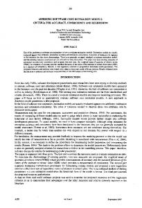
It is preferable that these (above) fuzzy sets satisfy the normal condition (NC), i.e., they form a fuzzy partition and each of them is convex and normal (Idri and Abran, 2001). The use of fuzzy sets to represent categorical data, such as very low and low, mimics the way in which the humanmind interpret these values, and consequently, it allows us to deal with vagueness, imprecision and uncertainty in the case(s) identification step. Another advantage of the proposed Fuzzy Analogy approach is that it takes into account the importance of each selected attribute in the case(s) identification step. Since all selected attributes do not necessarily have the same influence on the software project effort, we are required to indicate the weights (uk) associated with all the selected attributes in the case(s) identification step. In order to illustrate the case(s) identification step, we utilize the COCOMO’81 historical software projects data set. Each software project in the data set is described by 17 attributes, which are declared as relevant and independent (Boehm, 1981). Among these, the DATA cost driver is measured by four linguistic values, i.e., low, nominal, high, and very high. These linguistic values are represented by classical intervals in the original version of the COCOMO’81. Because of the advantages of representation (especially linguistic values) by fuzzy sets rather than classical intervals, we have proposed to use the representation given in Figure 3.2. The weight
associated to the DATA cost driver, i.e., udata, is equal to 1.23, and is evaluated by its productivity ratio1 . Low
Nominal
Very High
High
1
5 10 15
55
100
155
550
1000
1550
D/P
Fig. 3.2: Membership functions of fuzzy sets defined for the DATA cost driver (Idri et al., 2000)
3.5.2 Retrieval of Similar Cases This step is based on the preferred choice of a software project similarity measure. This selection is obviously very critical since it will influence which analogies or similar cases are extracted from the data set. The similarity of two software projects, which are described and characterized by a set of attributes, is often evaluated by measuring the distance between these two projects through their sets of attributes. Thus, two projects are considered dissimilar if the differences between their respective sets of attributes are clear and obvious. It is important to note that the similarity of two software projects also depends on their environment, i.e., projects that are similar in a specific type of environment may not necessarily be similar in other environments. Hence, according to Fenton’s definitions (Fenton and Pfleeger, 1997), a similarity measure should be considered as an external process attribute and, consequently, one which can only be measured indirectly. The technique by which the similarity of software projects is gauged is fundamental to the estimation of software development effort by analogy, and a variety of approaches have been proposed in the literature (Kolodner, 1993;Shepperd et al., 1996; Shepperd and Schofield, 1997) found three major inadequacies while investigating similarity measures: (1) that they are computationally intensive, and, consequently, many CBR systems 1 The productivity ratio is the software project’s productivity ratio expressed by the ratio of the Delivered Source Instructions by Man-Months for the best possible attribute rating to that of its worst possible variable rating, assuming that all the ratings for all other attributes remain constant.
have been developed, such as ESTOR (Vicinanza and Prietulla, 1990) and ANGEL (Shepperd et al., 1996), (2) that the algorithms are intolerant of noise and of irrelevant features, (3) probably the most critical, is that they do not deal well with categorical data other than binary-valued variables. However, in the software metrics domain, specifically in the context of software cost estimation models, many factors (linguistic variables in fuzzy logic), such as the experience of programmers and the complexity of modules, are measured on an ordinal (or nominal) scale composed of qualifications such as very low and low (linguistic values in fuzzy logic); these categorical data are represented by classical intervals (or step functions). Hence, no project can occupy more than one interval. This is a serious problem in that it can lead to a great difference in effort estimations in the case of similar projects with a small incremental size difference, since each would be placed in a different interval of a step function (Idri et al., 2000). To overcome the above-mentioned limitation, we have used fuzzy sets with a membership function rather than classical intervals to represent the categorical data. Based on the use of such a representation, we have proposed a set of new similarity measures (Idri and Abran, 2000). These measures evaluate the overall similarity, d(P1,P2), of two projects P1 and P2 by combining the individual similarities of P1 and P2 associated with the various linguistic variables (attributes) (Vj) describing P1 and P2, i.e., d v ( P1 , P2 ) (Fig. 3.3). j
Individual similarities of two projects P1 and P2, d v (P1 , P2 ) : The first j
step consists of calculating the similarity of P1 and P2 according to each individual attribute with a linguistic variable Vj, d v j ( P1 , P2 ) . Since each Vj is measured by fuzzy sets, d v j ( P1 , P2 ) should express the fuzzy equality according to Vj of P1 and P2. The associated fuzzy set then must have a membership function with two variables, i.e., Vj (P1) and Vj (P2). In the context of fuzzy set theory, this type of fuzzy set is referred to as a fuzzy relation. Such a fuzzy relation can represent an association or a correlation between elements of the product space. In our study, the association that will be represented by this fuzzy relation is the statement ‘P1 and P2 are approximately equal according to Vj’. We denote this fuzzy relation by v
R ≈ j , a combination of a set of fuzzy relations R≈v,jk . Each R≈v,jk represents v j the equality of Vj according to one of its linguistic values Ak . Hence, R≈,jk
represents the fuzzy if-then rule, where the premise and the consequence consist of the fuzzy proposition as shown below. v
R≈ ,j k : if V j ( P1 ) is Akj then V j ( P2 ) is Akj
(3.1)
RBASE
d v ( P1 , P2 ) 1
RBASE_V1
RBASE_V2
Aggregation
Aggregation
P1
d v ( P1 , P2 ) 2
P2
all most d(P1, P2) many .. there exists
d v ( P1 , P2 ) M
RBASE_VM
Aggregation
Fig. 3.3 Summarizes the process for computing the various measures.
Therefore, for each variable Vj, we have a rule base (RBASE_Vj) which contains the same number of fuzzy if-then rules as the number of fuzzy sets defined for Vj. Each RBASE_Vj expresses the fuzzy equality of two software projects according to Vj, d v j ( P1, P2 ) . When we consider all variables Vj, we obtain a rule base (RBASE) which contains all rules associated with all variables. RBASE expresses the fuzzy equality of two software projects according to all variables Vj, d(P1, P2). d v j ( P1, P2 ) is defined by combining all fuzzy rules in DBASE_Vj to obtain one fuzzy relation vj
( R ≈ ) which represents DBASE_Vj. The combination of the fuzzy if-then v
v j rules, R≈,jk , into a fuzzy relation, R ≈ , is called as aggregation. The way this is done is different for the various types of fuzzy implication functions adopted for the fuzzy rules. These fuzzy implication functions are based on distinguishing between two basic types of implication (Jager, 1995)): (1) the fuzzy implication which complies with the classical conjunction, and
(2) the fuzzy implication which complies with the classical implication. Using this basic distinction of the two types of fuzzy implication, we have obtained three equations for dv j ( P1, P2 ) : min( µ A ( P1 ), µ A ( P2 )) max k max − min aggregation ∑ µ A ( P1 ) × µ A ( P2 ) d v ( P1 , P2 ) = k sum − product aggregation max(1 − µ A ( P1 ), µ A ( P2 )) min k min − Kleene − Dienes aggregation j k
j k
j k
(3.2)
j k
j
j k
(3.3)
j k
(3.4)
In the context of the above equations, d v j ( P1, P2 ) = 1 implies a perfect similarity between P1 and P2 according to Vj; d v j ( P1, P2 ) = 0, a total absence of similarity; and 0 < d v j ( P1, P2 ) < 1, a partial similarity. Overall similarity of two projects P1 and P2, d(P1 ,P2) : To evaluate the overall similarity of P1 and P2, the individual similarities d v j ( P1 , P2 ) are ag-
gregated using Regular Increasing Monotone (RIM) linguistic quantifiers such as all, most, many, at-most α or there exists. The choice of the appropriate RIM linguistic quantifier, Q, depends on the characteristics and the needs of each environment. It indicates the proportion of individual distances that we feel is necessary for a good evaluation of the overall project similarity distance. The use of a RIM quantifier to guide the evaluation of the overall similarity essentially implies that the more individual similarities are satisfied, the greater is the overall similarity of the two software projects. The overall similarity of P1 and P2 , i.e., d(P1 ,P2), is given by one of the following formulas (Idri and Abran, 2001b): all of (d v j ( P1 , P2 )) most of (d v j ( P1 , P2 )) d ( P1 , P2 ) = many of (d v j ( P1 , P2 )) .... there exists of (d v ( P1 , P2 )) j
(3.5)
The following formal procedure is used to evaluate the overall similarity. First, the linguistic quantifier, Q, is used to generate an Ordered
Weight Averaging (OWA) weighting vector W (w1, w2, ..., wM) of dimension M (the number of variables describing the software project), such that all the wj are in the unit interval and their sum is equal to 1. Second, we calculated the overall similarity, d(P1, P2), by means of the following equation: M
d ( P1 , P2 ) = ∑ w j ( P1 , P2 ) d v ( P1 , P2 ) j
j =1
(3.6)
where, d v ( P1 , P2 ) is the jth largest individual distance. j
The procedure used for generating the weights, wj(P1,P2), from the linguistic quantifier Q is given by (Yager, 1996; Yager and Kacpruzyk, 1997): j
∑ uk
j −1
∑ uk
w j ( P1 , P2 ) = Q( k =1 ) − Q ( k =1 ) (3.7) T T where, uk is the importance weight associated with the kth variable describing the software project, and T is the total sum of all importance weights uk. We note that the weights wj(P1,P2) used in Formula (3.6) will generally be different for each (P1, P2). This is due to the fact that the ordering of the individual distances d v ( P1 , P2 ) will be different, leading to j
different uk values. Axiomatic validation of the similarity measures: As new measures are proposed, it is logical to ponder as to whether (or not) they capture the attribute they claim to describe. This allows us to choose the best measures from a very large number of software measures for a given attribute. However, validation of software measures is one of the most misunderstood procedures in the software measurement area. For example, “what constitutes is a valid measure?” A number of authors in the software measurement engineering domain have attempted to answer this question (Fenton et Pfleeger, 1997; Jacquet and Abran, 1998; Kitchenham et al., 1995; Zuse, 1994, 1999). However, the validation problem has to-date been tackled from different points of view (mathematical, empirical, etc.), and by interpreting the expression “metrics validation” differently; as suggested by Kitchenham et al: ‘What has been missing so far is a proper discussion of relationships among the different approaches’ (Kitchenham et al., 1995). Beyond this interesting issue, we use Fenton’s definitions to validate the two measures, d v j ( P1, P2 ) and d(P1,P2) (Fenton et Pfleeger, 1997), i.e.,
Validating a software measure is the process of ensuring that the measure is a proper numerical characterization of the claimed attribute by showing
that the representation condition is satisfied. This is validation in the narrow sense, implying that it is internally valid. If the measure is a component of a valid prediction system, the measure is valid in the wide sense. In this section, we deal with the validation of d v j ( P1, P2 ) and d(P1, P2) in the narrow sense. The measures, d v j ( P1, P2 ) and d(P1,P2), satisfy the representation condition if they do not contradict any intuitive notions about the similarity of P1 and P2. Our initial understanding of the similarity of projects will be codified by a set of axioms. This axiom-based approach is common in many sciences. For example, mathematicians learned about the world by defining axioms for geometry. Then, by combining axioms and using their results to support or refute their observations, they expanded their understanding and the set of rules that govern the behavior of objects. We present below, a set of axioms that represents our intuition about the similarity attribute between software projects and we check whether or not the two measures, d v j ( P1, P2 ) and d(P1,P2), satisfy these axioms. We also present a set of axioms that represent our intuition about the similarity attribute of two software projects and we resume, in Table 3.1, the results of the axiomatic validation of the two measures, d v j ( P1, P2 ) and d(P1, P2) (Idri and Abran, 2001). Axiom 1 (specific to the d v ( P, Pi ) measure): j
The similarity of two projects, according to a variable Vj, is not null if and only if these two projects have a degree of membership different from 0 to at least one same fuzzy set of Vj
d v j (P,Pi ) ≠ 0 iff ∃ Akj such that µ A j (P) ≠ 0 and µ A j (Pi ) ≠ 0 k
k
Axiom 2 We expect any measure S of the similarity of two projects to be nonnegative: S(P1, P2) ≥ 0; S(P, P) > 0 Axiom 3 The degree of similarity of any project to P must be lower or equal than the degree of similarity of P to itself: S(P, Pi) ≤ S(P, P)
Axiom 4 We expect any measure, S, of the similarity of two projects to be commutative: S(P1, P2)= S(P2, P1) d v (P, Pi ) /d(P, Pi) j
Axiom 1 Axiom 2 Axiom 3 Axiom 4
max-min Yes/ Yes/Yes Yes/Yes Yes/Yes
sum-product Yes/ Yes/Yes No/No Yes/Yes
Kleene-Dienes No/ Yes/Yes Yes /Yes if NC2 No/No
Table 3.1 Results of the validation of the distance d v (P, Pi ) and d (P, Pi) j
By observing the results of this validation, which takes into account the four axioms (Table 3.1), we conclude that d v j ( P, Pi ) using the max-min aggregation respects all the axioms (and consequently, so does d(P,Pi)). Hence, according to Fenton (Fenton et Pfleeger, 1997), this is a valid similarity measure in the narrow sense. d v j ( P, Pi ) , using the sum-product aggregation does not satisfy Axiom 2. Although Axiom 3 is interesting, we will retain the sum-product aggregation in order to be validated in the wide sense. There are three reasons for this decision (Idri and Abran, 2001): • The difference between d v j ( P, Pi ) and d v j ( P , P ) is not obvious if the fuzzy sets associated with Vj satisfy the normal condition. We can show that this difference, in the case where d v j ( P, Pi ) is higher than d v j ( P , P ) , is in the interval [-1/8, 0].
• Sum-product aggregation respects the other axioms, specifically Axiom 1. • As was noted by Zuse (Zuse, 1998), validation in the narrow sense, contrary to validation in the wide sense, is not yet widely accepted and mostly neglected in practice.
A tuple of fuzzy sets (A1, A2, .., AM) satisfies the normal condition (NC) if (A1, A2, .., AM) is a fuzzy partition and each Ai is normal and convex
2
d v j ( P, Pi ) , using min-Kleene-Dienes aggregation does not satisfy Axi-
oms 1 and 4. Although it satisfies Axioms 2 and 3, we rejected it because of Axiom 1. In our study, Axiom 1 represents the definition of the similarity of two software projects according to a fuzzy variable. Consequently, d v j ( P, Pi ) using min-Kleene-Dienes was not be used in the empirical validation of the Fuzzy Analogy approach. 3.5.3 Case adaptation
The objective of this step is to derive an estimate for the new project by using the known effort values of similar projects. There are two issues that need to be addressed. First, the choice of how many similar projects should be used in the adaptation? Second, how to adapt the chosen analogies in order to generate an estimate for the new project? In the literature, one can notice that there is no clear rule to guide the choice of the number of analogies, k. Shepperd et al. have tested two strategies to calculate the number k, by setting it to a constant value (they explored values between 1 and 5), or by determining it dynamically as the number of projects that fall within distance (d) of the new project (Kadoda et al., 2000). In contrast, Briand et al. have used a single case or analogy (Briand et al., 2000). Furthermore, Angelis and Stamelos have tested a number of analogies in the range of 1 to 10 when studying the calibration of the analogy procedure for the Albrecht’s dataset (Angelis and Stamelos, 2000). The results obtained from these empirical research efforts seemed to favour the case where k is lower than 3. Fixing the number of analogies for the case adaptation step is considered here neither as a requirement nor as a constraint. The principle of this approach is to take only the first k projects that are similar to the new project. Let us suppose that the distances between the first three projects of one dataset (P1, P2, P3) and the new project (P) are respectively: 3.30, 4.00 and 4.01. When we consider k equal to 2, we use only the two projects P1 and P2 in the calculation of an estimate of P. Project P3 is not considered in this case although there is no clear or obvious difference between d(P2, P) = 4.00, and d(P3, P) = 4.01. We believe that the use of the number k relies on the use of the classical logic principle, i.e., the transition from one situation (contribution in the estimated cost) to the following (no contribution in the estimated cost) is abrupt rather than gradual.
In Fuzzy Analogy, we propose a new strategy to select projects that will be used in the adaptation step. This strategy is based on the distances d(P, Pi) and the definition adopted in the studied environment for the proposition ‘Pi is closely similar project to P’. Intuitively, Pi is closely similar to P if d(P,Pi) is in the vicinity of 1 (0 in the case of the Euclidean distance similarity measure). A better way to represent the value ‘vicinity of 1’ is by using a fuzzy set defined in the unit interval [0, 1]. Indeed, this fuzzy set defines the ‘closely similar’ qualification adopted in the environment. Figure 3.4 demonstrates a possible representation for the value ‘vicinity of 1’. In this example all projects that have d(P,Pi) greater than 0.5 contribute to the estimated cost of P; the contribution of each Pi is weighted by µvicinity of 1(d(P,Pi)). 1 µvicinity of 1(x)
0.5
1
Fig. 3.4 A possible definition of the value ‘vicinity of 1’
The second issue in the case adaptation step is to generate an estimate for the new project by adapting the information gained from the chosen analogies. The most common solutions use the (weighted) mean or the median of the k chosen analogies. In the case of weighted mean, the weights can be the similarity distances or the ranks of the projects. In the case of the proposed Fuzzy Analogy approach, we use the weighted mean of all known effort projects in the dataset. The weights are the values of the membership function defining the fuzzy set ‘vicinity of 1’. The formula is then given by: N
Effort ( P) =
∑µ i =1
vicinity of 1
(d ( P, Pi )) × Effort ( Pi )
N
∑µ i =1
vicinity of 1
(3.8)
(d ( P, Pi ))
The primary advantage of our adaptation approach is that it can be easily configured by defining the value ‘vicinity of 1’ according to the needs of each development environment. An interesting situation arises when µvicinity of 1(x) = x in Formula (3.8), since it gives exactly the ordinary weighted
average. This property will be used in the validation of our approach on the COCOMO’81 dataset.
3.6 Empirical results The empirical results of applying the Fuzzy Analogy approach to the COCOMO’81 data set, are obtained by using the F_ANGEL tool, which is a software prototype that we have developed in order to automate the Fuzzy Analogy approach. In a broad sense, it can be viewed as a fuzzification of the classical analogy-based estimation tool, ANGEL, as developed by Shepperd et al. (Shepperd et al., 1996; Shepperd and Schofield, 1997). The results of our empirical validations were compared with those of three other cost estimation models, i.e., classical analogy, the original intermediate COCOMO’81, and ‘fuzzy’ intermediate COCOMO’81 (Boehm, 1981; Idri et al., 2000). The accuracy of the estimates is evaluated by using the magnitude of relative error (MRE), which is defined as: MRE =
Effortactual − Effortestimated Effort actual
(3.9)
The MRE is calculated for each project in the dataset. In addition, we use the prediction level measure, Pred(p), which has often been used in the literature. It is defined by: Pr ed ( p ) =
k N
(3.10)
where, N is the total number of observations, k is the number of observations with a MRE less than or equal to p. A common value for p is 0.25, and in our evaluations, we use p equal to 0.20 since it was used for evaluation of the original version of the intermediate COCOMO’81 model. The Pred(0.20) gives the percentage of projects that were predicted with a MRE equal or less than 0.20. Other four quantities are used in this evaluation: min of MRE, max of MRE, standard deviation of MRE (SDMRE), and mean MRE (MMRE). The original intermediate COCOMO’81 database was chosen as the basis for this validation (Boehm, 1981). It contains 63 software projects. Each project is described by 17 attributes: (1) software size, measured in KDSI (Kilo Delivered Source Instructions), (2) project mode, defined as either ‘organic’, ‘semi-detached’, or ‘embedded’, and the remaining (3)(15) cost drivers are generally related to the software environment. Each cost driver is measured on a scale composed of six qualifications: very low,
low, nominal, high, very high, and extra-high. It seems that this scale is ordinal, but an analysis indicates that one of the 15 cost drivers (SCED attribute) is only assessed to be nominal. This does not cause any problem for the proposed Fuzzy Analogy technique, because it deals with these six qualifications as linguistic values rather than categorical data. In the original intermediate COCOMO’81, the assignment of linguistic values to the 15 cost drivers used conventional quantization, such that the values belonged to classical intervals (see (Boehm, 1981), pp. 119). Due to the various advantages of representation by fuzzy sets as compared to representation by classical intervals, the 15 cost drivers should be represented by fuzzy sets. Among these, we have retained 12 attributes that we had already fuzzified elsewhere (Idri et al., 2000). The other attributes are not studied because their relative descriptions proved insufficient. In this evaluation, we assumed that only these 12 cost drivers (see Figure 3.5) describe all the COCOMO ‘81 software projects The original COCOMO’81 database contains only the effort multipliers; therefore, our evaluation of the proposed Fuzzy Analogy technique will be based on three 'fuzzy' data sets deduced from the original COCOMO’81 database. Each of these three 'fuzzy' data sets contains 63 projects with the values necessary to determine the 12 linguistic values associated to each project. These 12 linguistic values were used to evaluate the similarity between software projects. One of these three fuzzy data sets is considered as a historical dataset, while the other two are perceived as the current datasets containing the new projects. The results obtained by using only the max-min aggregation to evaluate the individual distances (Formula (3.2)) are presented in Table 3.2. We have not presented results of using the sum-product aggregation (Formula (3.3)) for two primary reasons (Idri and Abran, 2001): • Under what we have referred as normal condition, the max-min and sum-product aggregations yielded approximately similar results, and this was the case for the COCOMO’81 database. • The sum-product aggregation does not satisfy all (previously discussed) established axioms .
α-RIM
Max 1/100 1/30 1/15 1/10 1/7 1/3 1 3 7 10 15 30 100 Min
Pred(0.20) (%0) 4.76 4.76 4.76 4.76 4.76 4.76 6.34 6.34 6.34 9.52 15.87 38.09 74.60 92.06 92.06
Dataset #1 MMRE SDMRE (%) (%) 1801.48 2902.94 1798.85 2897.77 1792.70 2885.74 1783.91 2868.69 1757.13 2851.77 1763.86 2830.24 1714.20 2737.66 1550.89 2455.21 1168.24 1889.23 633.99 1215.81 371.84 802.30 143.92 337.76 20.40 42.06 4.06 9.05 4.03 9.17
Dataset #2 Pred(0.20) MMRE SDMRE (%) (%) (%) 4.76 2902.49 1807.17 4.76 2894.28 1803.41 4.76 2875.26 1794.69 4.76 2848.44 1782.32 4.76 2822.64 1770.06 4.76 2788.70 1754.48 6.34 2648.90 1687.68 3.17 2258.36 1485.66 9.52 1571.48 1063.19 14.28 830.79 526.57 20.63 525.45 305.98 36.50 284.20 140.68 77.77 160.38 51.67 84.12 30.37 10.49 87.30 29.12 8.53
Table 3.2 Results of the evaluation of Fuzzy Analogy
‘fuzzy’/classical intermediate COCOMO’81 Dataset #1 Dataset #2 Pred(20) (%) Min MRE (%) Max MRE (%) Mean MREi(%) Standard deviation MRE
62.14 0.11 88.60 22.50 19.69
68 0.02 83.58 18.52 16.97
46.86 0.40 3233.03 78.45 404.40
68 0.02 83.58 18.52 16.97
Classical analogy (Two datasets) Pred(0.20) K % 31.75 2 25.40 3 19.05 4 12.70 5 12.70 6
Table 3.3 Comparing classical analogy, ‘fuzzy’ and classical intermediate COCOMO’81 models (Idri et al., 2000).
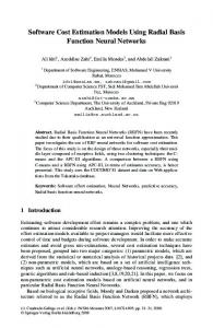
Generally speaking, for the overall distances, each project environment must define its appropriate quantifier by studying its specific features and requirements. Due to a lack of knowledge regarding the appropriate quantifier for the environment from which the COCOMO’81 data was collected, we utilized various quantifiers to combine the individual similarities, including all, there exists, and α-RIM linguistic quantifiers. An αRIM linguistic quantifier is defined by a fuzzy set in the unit interval with the membership function Q, given by: Q( r ) = r α α > 0 To compute the weights wj’s (Formula 3.7), importance of the weights uk’s associated with the 12 variables describing COCOMO’81 software projects, needs to be determined. For the same purpose, we used the productivity ratio, which is the project’s productivity ratio (expressed in Delivered Source Instructions by Man-Month) for the best possible variable rating to its worst possible variable rating, assuming that the ratings for all other variables remain constant (Fig. 3.5). Upon results-analysis of the empirical validation (Table 3.2), we observed that the accuracy of the estimates depended on the linguistic quantifier (α) used in the evaluation of the overall similarity between software projects. Hence, if we consider the accuracy measured by Pred(0.20) as a function of α, we notice that, in general, it is monotonously increasing relation according to α. This is because, our similarity measures are monotonously decreasing functions with respect to α. Subsequently, when α tends towards zero, it implies that the overall similarity will take into account fewer attributes amongst those describing the software projects. The minimum number of attributes that should be considered is one. This is the case when using the ‘max’ operator where the selected attribute is the one for which the associated individual distance is the maximum of all individual distances. As a consequence, the overall similarity will be higher because we are more likely to find in the COCOMO’81 data set at least one attribute for which the associated linguistic values are the same for the two projects. In contrast, when α tends to approach infinity it implies that the overall similarity will take into account many attributes amongst the ones describing the software projects. As a maximum, we may consider all attributes: this was the case when combining similarities with the ‘min’ operator. As consequence, the overall similarity will be minimal because we are more likely to find in the COCOMO’81 data set one attribute for which the associated linguistic values are different for the two projects.
It is important to note the soft aspects of the proposed Fuzzy Analogy approach. First, the appropriate weights associated with linguistic variables describing a software project (uk) can be chosen. These weights represent the importance of the variables in the environment. Second, we can choose the appropriate linguistic quantifier to combine the individual distances, and this linguistic quantifier is used to generate the weights, wj’s. These weights represent the importance associated with the individual distances when evaluating the overall distance. They depend upon the weights uk and the chosen linguistic quantifier. An interesting scenario arises when uk = wk. This occurs when the factor α = 1. As a consequence, Formula (3.7) yields the ordinary weighted average.
SCED
LEXP
DATA
TURN
VEXP
VIRT-MAJ
VIRT-MIN
STOR
AEXP
TIME
PCAP
ACAP
2,5 2 1,5 1 0,5 0
Fig. 3.5. Comparing productivity ratios for the 12 variables describing COCOMO’81 projects
Figure 3.6 shows the relation between α and the number of projects that have a MRE smaller than 0.20 (NPU20) for data set #2. The two bold lines respectively represent the minimum and the maximum accuracy of the Fuzzy Analogy method when it uses the min- and max-aggregation to combine individual similarities. The ‘max’ (‘min’) aggregation gives lower (higher) accuracy because it considers only one (all) attribute(s) in the evaluation of the similarity. In the case of the other α-RIM linguistic quantifiers (0 < α < ∞), the accuracy increases with α because additional attributes will be considered in the evaluation of the overall similarity. For example, a software project Pi which has an overall similarity with P different from zero when α is equal to 10, may have a null overall similarity when α is equal to 30. Due to this reason, it is not used in the estimation of the cost for α = 30.
NPU20 Min aggregation
60 55 50 45 40 35 30 25 20 15 10
Max aggregation
5 0 0
20
40
60
80
100
120
140
α
Fig. 3.6 α versus the number of projects of Dataset #2 with MRE