Fuzzy Geometric Programming Approach in Multi-objective ...

International Journal of

Operations Research International Journal of Operations Research Vol. 12, No. 2, 021−035(2015)

Fuzzy Geometric Programming Approach in Multi-objective Multivariate Stratified Sample Surveys in Presence of Non-Response Shafiullah*, Irfan Ali and Abdul Bari Department of Statistics and Operations Research, Aligarh Muslim University Aligarh, UP, INDIA Received October 2014; Revised October 2014; Accepted January 2015

Abstract  In this paper, we have formulated the problem of non-response in multivariate stratified sample surveys as a Multi-Objective Geometric Programming problem (MOGPP). The fuzzy programming approach has described for solving the formulated MOGPP. The formulated MOGPP has been solved and the solution is obtained. The obtained solution is the dual solution corresponding to the multi-objective multivariate stratified sample surveys in presence of non-response. Afterward with the help of dual solution of formulated MOGPP and primal-dual relationship theorem the optimum allocation of sample sizes of respondents and non respondents are obtained. A numerical example is given to illustrate the procedure.

Keywords  geometric programming, fuzzy programming, multi-objective optimization, non-response, optimum allocation, multivariate stratified sampling

1.

INTRODUCTION

In stratified sampling heterogeneous population is converted into a homogeneous population by dividing it into homogeneous stratum. The maximum precision will be obtained with the best choices of the sample sizes. The problem of optimum allocation in stratified random sampling for univariate population is well known in sampling literature; see for example Cochran (1977) and Sukhatme et al. (1984). In multivariate stratified sample survey the problem of non-response can appear when the required data are not obtained. The problem of non-response may occur due to the refusal by respondents or they are not at home making the information of sample inaccessible. The problem of non-response occurs in almost all surveys. The extent of non- response depends on various factors such as type of the target population, type of the survey and the time of survey. For dealing the problem of non-response the population is divided into two disjoint groups of respondents and non respondents. For the stratified sampling it may be assumed that every stratum is divided into two mutually exclusive and exhaustive groups of respondents and non respondents. Hansen and Hurwitz (1946) presented a classical non-response theory which was first developed for the survey in which the first attempt was made by mailing the questionnaires and a second attempt was made by personal interview to a sub sample of the non respondents. They constructed the estimator for the population mean and derived the expression for its variance and also worked out the optimum sampling fraction among the non respondents. El-Badry (1956) further extended the Hansen and Hurwitz’s technique by sending waves of questionnaires to the non respondent units to increase the response rate. The generalized El-Badry’s approach for different sampling design was given by Foradari (1961). Srinath (1971) suggested the selection of sub samples by making several attempts. Khare (1987) investigated the problem of optimum allocation in stratified sampling in presence of non-response for fixed cost as well as for fixed precision of the estimate. Khan et al. (2008) suggested a technique for the problem of determining the optimum allocation and the optimum sizes of subsamples to various strata in multivariate stratified sampling in presence of non-response which is formulated as a nonlinear programming problem (NLPP). Varshney et al. (2011) formulated the multivariate stratified random sampling in the presence of non-response as a multi-objective integer nonlinear programming problem and a solution procedure is developed using lexicographic goal programming technique to determine the compromise allocation. Fatima and Ahsan (2011) address the problem of optimum allocation in stratified sampling in the presence of non-response. Raghav et al. (2014) have discussed the various multi-objective optimization techniques in the multivariate stratified sample surveys in case of non-response Geometric programming (GP) is a smooth, systematic and an effective non-linear programming method used for solving problems of sample surveys and engineering design that takes the form of convex programming. The convex * Corresponding author’s email: [email protected]

22 Shafiullah and Bari: Fuzzy Geometric Programming Approach in Multi-objective Multivariate Stratified Sample Surveys in Presence of Non - Response IJOR Vol. 12, No. 2, 021−035 (2015)

programming problems occurring in GP are generally represented by an exponential or power function. GP has certain advantages over the other optimization methods because it is usually much simpler to work with the dual than the primal one. The degree of difficulty (DD) plays a significant role for solving a non-linear programming problem by GP method. Geometric Programming (GP) has been known as an optimization tool for solving the problems in various fields. Duffin, Peterson and Zener (1967) and also Zener (1971) have discussed the basic concepts and theories of GP with application in engineering in their books. Beightler, C.S., and Phililps, D.T., also published a famous book on GP and its application in (1976). Engineering design problems was also solved by Shiang (2008) and Shaojian et al. (2008) with the help of GP. Davis and Rudolph (1987) applied GP to optimal allocation of integrated samples in quality control. Ahmed and Charles (1987) applied geometric programming to obtain the optimum allocations in multivariate double sampling. Maqbool et al. (2011), Shafiullah et al. (2013) have discussed the geometric programming approach for obtaining the optimum allocations in multivariate two-stage and three-stage sample surveys respectively. In many real-world decision-making problems of sample surveys, environmental, social, economical and technical areas are of multiple-objectives problems. Multi-objective optimization problems differ from single-objective optimization. It is significant to realize that multiple objectives are often non-commensurable and in conflict with each other in optimization problems. The fuzzy goal is defined as the objective which can be obtained within exact target value. The multi-objective models with fuzzy objectives are more realistic than deterministic of it. The concept of fuzzy set theory was firstly given by Zadeh (1965). Later on, Bellman and Zadeh (1970) used the fuzzy set theory to the decision-making problem. Tanaka (1974) introduces the objective as fuzzy goal over the α-cut of a fuzzy constraint set and Zimmermann (1978) gave the concept to solve multi-objective linear-programming problem. Biswal (1992) and Verma (1990) developed fuzzy geometric programming technique to solve multi-objective geometric programming (MOGP) problem. Islam (2005, 2010) has discussed modified geometric programming problem and its applications and also another fuzzy geometric programming technique to solve MOGPP and their applications. Fuzzy mathematical programming has been applied to several fields. In this paper, we have formulated the problem of non-response in multivariate stratified sample surveys as a multi-objective geometric programming problem (MOGPP). The fuzzy geometric programming approach has described for solving the formulated MOGPP and optimum allocation of sample sizes of respondents and non respondents are obtained. A numerical example is given to illustrate the procedure. 2.

FORMULATION OF THE PROBLEM In stratified sampling the population of N units is first divided into L non-overlapping subpopulation called strata, of L

sizes N 1 , N 2 ,..., N h ,..., N L with ∑ N h = N

and

the

respective

sample

sizes

within

strata

are

denoted

by

h =1 L

n1 , n 2 ,..., n h ,..., n L with

∑ n h = n. h =1

Let for the h th stratum: : denote the stratum size.

Nh

Y h : Stratum mean.

S h2

: Stratum variance.

Wh =

Nh : Stratum weight. N

N h1 : be the sizes of the respondents.

N h 2 = N h − N h1 : be the sizes of non respondents groups.

n h : Units are drawn from the h th stratum. Further let out of nh , nh1 units belong to the respondents group. n h 2 = n h − n h1 : Units belong to the non respondents group. L

n = ∑ n h : The total sample size. h =1

A more careful second attempt is made to obtain information on a random subsample of size rh out of n h 2 non respondents for the representation from the non respondents group of the sample. rh =

nh 2 ; h = 1, 2,..., L : Subsamples of sizes at the second attempt to be drawn from nh 2 non–respondent group of the h th kh

stratum. Where k h ≥1 and

1 denote the sampling fraction among non respondents. kh

1813-713X Copyright © 2015 ORSTW


Since N h1 and N h 2 are random variables hence their unbiased estimates are given as n N Nˆ h1 = h1 h : Unbiased estimates of the respondents group. nh n N Nˆ h 2 = h 2 h : Unbiased estimate of the non respondents group. nh

j th characteristic measured on the n h1 respondents at the first attempt.

y jh1 ; j = 1,..., p : denote the sample means of

y jh 2( rh ) ; j = 1,..., p : denote the rh sub sampled units from non respondents at the second attempt.

Using the estimator of Hansen and Hurwitz (1946), the stratum mean Y may be estimated by y jh ( w) =

jh

for j th characteristic in the h th stratum

n h1 y jh1 + n h 2 y jh 2( rh )

(1)

nh

It can be seen that y jh(w) is an unbiased estimate of the stratum mean Y

jh

of the h th stratum for the j th characteristic

with a variance. W2 S2 W2 S2  1 1  2  S jh + h 2 jh 2 − h 2 jh 2 v y jh ( w) =  −  rh nh  nh N h 

(

)

(2)

where S 2jh is the stratum variance of j th characteristic in the h th stratum; j = 1,2,..., p, h = 1,2,..., L. given as: S 2jh =

(

1 Nh ∑ y jhi − Y N h − 1 i =1

)

2

jh

where y jhi denote the value of the i th unit of the h th stratum for j th characteristic. Y jh =

y jhi .

of

S 2jh 2

is the stratum variance of the j

th

characteristic in the h S 2jh 2 =

Y

jh 2

1 ˆ N h2

=

Nˆ h 2

∑ y jhi

is the stratum mean of

1

Nˆ h 2

Nˆ h 2 − 1

i =1

th

1 Nh

Nh

∑ y jhi : is the stratum mean i =1

stratum among non respondents, given by:

∑ (y jhi − Y jh 2 ) , 2

y jhi among non respondents. Wh 2 =

i =1

Nh2 Nh

is stratum weight of non

respondents in h th stratum. If the true values of S 2jh and S 2jh 2 are not known they can be estimated through a preliminary sample or the value of L

some previous occasion, if available, may be used. Furthermore, the variance of y j ( w) = ∑ Wh y jh ( w) , (ignoring fpc) is given h =1

as:

(

)

V y j ( w) =

where

(

L

L

Wh2 S 2jh − Wh 2 S 2jh 2

h =1

h =1

nh

∑ Wh2 v (y jh ( w) ) = ∑

y j ( w) is an unbiased estimate of the overall population mean

)+

Yj

L

Wh2Wh 2 S 2jh 2

h =1

rh

∑

(3)

(

of the j th characteristic and V y jh (w)

)

is as

given in Eqn.2. Assuming a linear cost function the total cost C of the sample survey may be given as: L

L

h =1

h =1

L

C = ∑ c h0 n h + ∑ c h1n h1 + ∑ c h 2 n h 2 h =1

p

where ch 0 = the per unit cost of making the first attempt, ch1 = ∑ c jh1 is the per unit cost for processing the results of all j =1

the p characteristics on the nh1 selected units from respondents group in the h th stratum in the first attempt and p

c h 2 = ∑ c jh 2 is the per unit cost for measuring and processing the results of all the p characteristics on the rh units selected j =1

from the non respondents group in the h th stratum in the second attempt. Also, c jh1 and c jh 2 are per unit costs of measuring the j th characteristic in first and second attempts respectively. As nh1 is not known until the first attempt has been made, the quantity Wh1nh1 may be used as its expected value. The total expected cost Cˆ of the survey may be given as: 1813-713X Copyright © 2015 ORSTW


L

L

h =1

h =1

Cˆ = ∑ (c h 0 + c h1Wh1 )nh + ∑ c h 2 rh

(4)

The problem therefore reduces to find the optimal values of sample sizes of respondents nh* and non-respondents rh* which are expressed as:

(

)+

Wh2Wh 2 S 2jh 2   nh rh h =1 h =1   Subject to , j = 1, 2, … , p L L  ∑ (c h 0 + ch1Wh1 )nh + ∑ c h 2 rh ≤ C 0  h =1 h =1  n h , rh ≥ 0 and n h , rh are integers 

( )

L

Min f 0 j = ∑

3.

Wh2 S 2jh − Wh 2 S 2jh 2

L

∑

(5)

MOGPP FORMULATION OF SAMPLE SURVEYS PROBLEM IN PRESENCE OF NON-RESPONSE

Geometric programming always transforms the primal problem of minimizing a “posynomial” subject to “posynomial” constraints to a dual problem of maximizing a function of the weights on each constraint. Posynomial functions can be defined as polynomials in several variables with positive coefficients in all terms and the power to which the variables are raised can be any real number. The mathematical formulation of problem (5) can be rewritten as: L ψ L ψ  1h 2h Min f 0 j = ∑

+

∑

   Subject to , j = 1,2,..., p L L  C n + C' r ≤ C ∑ h h ∑ hh 0  h =1 h =1  n h , rh ≥ 0 and n h , rh are int egers  h =1

nh

where C h = (c h 0 + c h1Wh1 ), C ' h = c h 2 ,

h =1

rh

(

(6)

)

If q = 1, let the function ψ qh be define as, ψ 1h = Wh2 S 2jh − Wh 2 S 2jh 2 , and if q = 2, then ψ 2 h = Wh2Wh 2 S 2jh 2 , where q is the number of functions in objective function. The above expression (6) can be expressed in the standard Primal GPP as follows: f 0 j (n, r ), j =1,2,..., p   Subject f (n, r ) ≤ 1  n h , rh ≥ 0, h = 1, 2,⋯ , L  Max

L

where f0 j n, r = ∑

( )

h =1

ψ 1h nh

L

+

∑ h =1

ψ 2h rh

( )

, j = 1, 2,..., p and f n, r =

(7)

L

L

h =1

h =1

∑C h nh + ∑C h' rh are in the form of posynomial

functions, where the posynomial function is given as: L L  L L  f (n, r ) = ∑ ξ 1h ∏ n hp11h  + ∑ ξ 2h ∏ rhp12 h , ξ qh , ≥ 0 , n h , rh ≥ 0, q = 1, 2 h =1  h =1  h=1  h =1 

where ξ qh are normalized constants. If q = 1, let the function ξ qh be define as, ξ1h =

Ch C0

and if q = 2, then ξ 2 h =

(8) C 'h , C0

where q is the total number of functions in the constraint. If q be the number of terms in the problem. Then the number of posynomial terms in objective function f 0 j (n, r ) For the above problem of sample surveys, q = 2 as nh and rh are two different variables

can be denoted by qh. th

corresponding to the h strata. Therefore, the total number of posynomial terms for the discussed problem will be 2h and h= 1, 2,…, L. Similarly, the total numbers of posynomial terms corresponding to the primal constraint are denoted by 2h as n h and rh are two different variables and the exponents p 0 ih and p1ih are real constants corresponding to the objective functions and constraints functions respectively. The dual form of standard Primal MOGPP which is stated in (7) can be given as:



  (i)   q L  Subject ∑ ∑ w 0ih = 1 (ii )  j = 1, …, p i =1 h =1  q q L L  p0ih w 0ih + ∑ ∑ p1ih w1ih = 0 (iii)  ∑ ∑ i =1 h =1 i =1 h =1  w 0ih ≥ 0, w1ih ≥ 0, i = q and h = 1, …, L (iv )   where w0ih ' s and w1ih ' s are the dual variables corresponding to the objective functions and constraints functions. The above formulated MOGPP (9) can be solved in the following two-steps: Step 1: For the Optimum value of the objective function, the objective function always takes the form:   ψ Max v 0 j (w 0*i ) = ∏∏  ih  i =1 h =1  w 0ih  q

L

w 0 ih

  

 Coefficent of first term   v 0 j ( w0*i ) =   w1  

(∑ w' s in the

   q L  ξih  ∏∏   i =1 h =1  w1ih

w1

first constra int s )∑ w's in the

w1ih

  

q

 Coefficent of sec ond term   ×   w2   first constra int s

×

L

∑ ∑ w  i =1 h =1 1ih  q L   ∑ ∑ w1ih     i =1 h =1

w2

 Coefficent of last term   × ......×   wL  

(9)

wL

(∑ w' s in the last constra int s )∑ w's in the last constra int s

The Multi-Objective objective function for our problem is:

  ψ ih  ∏∏ i =1 h =1  w 0ih  q

where ξ1h =

Ch C0

L

and ξ2h =

C 'h C0

w 0 ih

  

   q L  ξih  ∏ ∏   i =1 h =1  w1ih

w1ih

  

q

L

∑ ∑ w  i = 1 h =1 1ih  q L w   ∑ ∑ 1ih     i =1 h =1

(10)

. ξqh are normalized constants.q = 1, 2. ; h = 1, 2,..., L. q

L

Step 2: The equations that can be used for MOGPP for the weights are given below: ∑ ∑ w0ih in the objective function= i =1 h=1

1(Normality condition ,see 9(ii)) and for each primal variable ni and ri q

having qh terms.

L

∑ ∑ (w0ih for each term in objective function )× (exponent on n h and rh in objective function )× i =1 h =1 q

L

∑ ∑ (w1ih for each term in constraints function )× (exponent on n h and rh in constraints function ) = 0 i =1 h =1

(Orthogonality condition, see 9(iii)) and w0ih ≥ 0, w1ih ≥ 0 (Positivity condition, see 9(iv)). 4.

FGP APPROACH IN SAMPLE SURVEYS IN PRESENCE OF NON- RESPONSE

The solution procedure to solve the problem (6) consists of the following steps: Step 1: Solve the MOPP as a single objective problem using only one objective at a time and ignoring the others. These solutions are known as ideal solution. Step 2: From the results of step-1, determine the corresponding values for every objective at each solution derived. With the values of all objectives at each ideal solution, pay-off matrix can be formulated as follows: f 01 ( n, r ) ( n (1) , r (1) ) ( n ( 2 ) , r (2 ) ) ⋮ (n ( j ) , r ( j ) ) ⋮ (n ( p ) , r ( p ) )

 f 01* ( n (1) , r (1) )   f 01 ( n ( 2 ) , r (2 ) )   ⋮  ( j) ( j)  f 01 ( n , r ) ⋮   f (n ( p ) , r ( p ) )  01

f 02 ( n, r )

⋯

f 0 j ( n, r )

f 02 ( n (1) , r (1) )

⋯

f 0 j ( n (1) , r (1) )

f 02* ( n ( 2 ) , r (2 ) )

⋯

f 0 j (n ( 2) , r ( 2) )

⋮ f 02 (n ( j ) , r ( j ) ) ⋮ f 02 ( n ( p ) , r ( p ) )

⋯ ⋯

⋮ f 0*j (n ( j ) , r ( j ) )

…

⋯ ⋯ ⋯ ⋯

⋮ ⋯ . f 0 j (n ( p ) , r ( p ) )

⋯

f 0 p (n, r ) f 0 p ( n (1) , r (1) )

  f 0 p ( n ( 2 ) , r (2 ) )   ⋮   ( j) ( j) f 0 p (n , r )   ⋮  * ( p) ( p) f 0 p ( n , r ) 

Here (n (1) , r (1) ), (n ( 2) , r (2 ) ), ⋯ , (n ( j ) , r ( j ) ), ⋯, (n ( p ) , r ( p ) ) are the ideal solutions of the objective functions 1813-713X Copyright © 2015 ORSTW


f 01 ( n (1) , r (1) ), f 02 ( n ( 2 ) , r ( 2 ) ) , ⋯ , f 0 j ( n ( j ) , r ( j ) ), ⋯ , f 0 p ( n ( p ) , r ( p ) ) .

So U j = Max {f 01 ( n (1) , r (1) ), f 02 ( n ( 2 ) , r ( 2 ) ) , ⋯ , f 0 p ( n ( p ) , r ( p ) )} and L j = f 0*j (n ( j ) , r ( j ) ), j =1,2,..., p .

[U

j

]

and L j be the upper and lower bonds of the j th objective function f 0 j (n, r ) , j = 1,2,.., p.

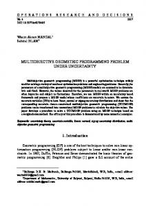
Step 3: The membership function for the given problem can be define as:

µj(

 0 , if f 0 j (n, r ) ≥ U j   U j (n, r ) − f 0 j (n, r ) f 0 j (n, r ) =  , if L j ≤ f 0 j (n, r ) ≥ U j , j = 1, 2, … , p  U j (n, r ) − L j (n, r )  1 , if f (n, r ) ≤ L 0j j 

)

(11)

µ j ( f 0 j (n, r ))

1

Figure 1: Membership function for minimization variance problem

( ( ))

The membership functions in Eqn. (11) i.e., µ j f0 j n, r , j = 1, 2,⋯ , p . Therefore the general aggregation function can

( )

{ (f

be defined as µ ɶ n, r = µ ɶ µ D

D

1

01

(n, r ) ) , µ ( f (n, r ) ) ,..., µ ( f (n, r ) )} . 02

2

0p

p

The fuzzy multi-objective formulation of the problem can be defined as: Max µ ~ (n, r )  D

  Subject to ∑ C1n h + ∑ C 2 rh ≤ 1; , j = 1,2,..., p h =1 h =1  n h , rh ≥ 0 and n h , rh are integers,  L

L

(12)

The problem to find the optimal values of ( n* , r * ) for this there are two types of fuzzy decision operators and they (1) (i) Fuzzy decision based on max-min operator (like Zimmermann’s approach (1978)). Therefore the problem (12) is reduced to the following problems according to max-min operator     L L ∑ C1 n h + ∑ C 2 rh ≤ 1;  h =1 h =1  n h , rh ≥ 0. and n h , rh are integers,   j = 1,2,..., p, 0 ≤ α ≤ 1. 

Max α Subject to µ j f 0 j (n,r ) ≥ α

(

)

(13)

(ii) Convex-fuzzy decision based on addition operator (like Tewari et al. (1987)). Therefore the problem (12) is reduced according to max-addition operator as



(

)

Max µ D n * , r * =

p

j =1

Subject to

L

L

h =1

h =1

(

)

p

U j − f 0 j (n, r )

j =1

U j −Lj

∑ µ j ( f 0 j (n, r )) = ∑

∑ C1n h + ∑ C 2 rh ≤ 1;

(

)

0 ≤ µ j f 0 j (n, r ) ≤ 1, and n h , rh ≥ 0 , n h , rh are integers and j = 1,2, ⋯ , p.

        

(14)

The above problem (14) reduces to

(

)

      L L  f j (n, r ) = ∑ C1 n h + ∑ C 2 rh ≤ 1;  h =1 h =1  n h , rh ≥ 0 and n h , rh are integers, j = 1,2,..., p.

p  U f 0 j (n, r )   j − Max µ D n * , r * = ∑   U j − L j  j =1  U j − L j Subject to

(

)

(

)

(

)

(15)

 f 0 j (n, r )   attain the minimum values. Therefore the problem (15) reduce  U j − L j 

The problem (15) maximizes if the function  into the problem (16) define as

     Subject to , j = 1,2,..., p. L L  f j (n,r ) = ∑ C1 nh + ∑ C 2 rh ≤ 1;  h =1 h =1  nh , rh ≥ 0 and nh , rh are integers,   f 0 j (n,r )   j =0   U j − L j  p

Min

∑

(16)

The problem (16) has been solved with the help of steps (1-2) discuss in section (3) and the corresponding solutions w*0i is the unique solution to the dual constraints, it will also maximize the objective function for the dual problem. Next, the solution of the primal problem will be obtained using primal-dual relationship theorem which is given below: Primal-dual relationship theorem: If w*0i is a maximizing point for dual problem (9), each minimizing points

(n1 , n2 , n3 , n4

and r1 , r2, r3 , r4

)

for primal problem (6) satisfies the system of equations:

( )

w0* j v w* ,  f 0 j (n, r ) =  wij ,   v L w0*i

( )

j ∈ J [0],   i ∈ J [L],  

(17)

where L ranges over all positive integers for which v L (w0*i )> 0 . The optimal values of respondents n h* and non-respondents rh* can be calculated with the help of the primal – dual relationship theorem (17). 5.

NUMERICAL ILLUSTRATION A numerical example is given to demonstrate the proposed method. The values of S 2jh 2 and S 2jh and are practically

unknown. Their values on some previous occasion may be used. It is assumed that the relative values of the stratum variances among the non respondents at the second attempt to the corresponding over all stratum variances are S 2jh 2 S 2jh

= 0.25

; h = 1, 2,…,L and j = 1,2,…, p. This ratio has been taken as 0.25 in the example for the sake of simplicity.

Practically this ratio may vary from stratum to stratum and from characteristic to characteristic. Consider a population of size N = 3850 divided into four strata. The two characteristics are defined on each unit of the population and the population means are to be estimated. The available information is shown in the given table.



h

Nh

S1h2

1

1214

4817.72

2

822

3 4

2 S 2h

wh1

wh 2

ch0

c h1

ch 2

8121.15

0.7

0.30

1

2

3

6251.26

7613.52

0.80

0.20

1

3

4

1028

3066.16

1456.4

0.75

0.25

1

4

5

786

6207.25

6977.72

0.72

0.28

1

5

6

Table 1: Data for four Strata and two characteristics For solving MOGPP by using fuzzy programming, we shall first solve the two sub-problems: Sub problem1: On substituting the table values in sub-problem 1, we have obtained the expressions given below:

456.3344 261.8965 209.5529 230.9097 + + + + n1 n2 n3 n4 11.10002688 2.75680566 3.492547875 4.866484 + + + r1 r2 r3 r4

Min f01 =

Subject to 0.00048n1 + 0.00068n2 + 0.0008n 3 + 0.00092n 4 + 0.0006r1 + 0.0008r2 + 0.001r3 + 0.0012r4 ≤ 1

(

nh ≥ 0 , rh ≥ 0 ; h = 1, 2,...,L The dual of the above problem (18) is obtained as: w max v(w 0*i ) =  456.3344 / w 01 01  ×  261.8965 / w 02    w 04  ×  11.100027 / w ×  230.9097 / w 04   05   

)

            

 ×  209.5529 / w w03     03    w 05 w 06  ×  2.756806 / w     06    w11 w12     w 07 w 08 0.00048     0.00068        ×  3.492548 / w 07 ×     ×  4.866484 / w 08  ×        w11     w12       w w w w   13    0.00092  14    0.0006  15    0.0008  16  0.0008 ×  ×    ×    ×     w13     w14     w15     w16           w17 w18       0.001 0.0012 ×  ×     w    w   17   18      × ((w11 +w12 +w13 +w14 +w15 +w16 +w17 +w18 )^(w11 +w12 +w13 +w14 +w15 +w16 +w17 +w18 )); w 02

( (

) )

(

(

) )

(

)

(

)

( (

) )

Subject to w 01 + w 02 + w 03 + w 04 + w 05 + w 06 + w 07 + w 08 = 1; (normality condition) − w 01 + w11 = 0   − w 02 + w12 = 0;  − w 03 + w13 = 0;   − w 04 + w14 = 0;  (orthogonality condition)  − w 05 + w15 = 0;  − w 06 + w16 = 0;   − w 07 + w17 = 0;  − w 08 + w18 = 0;   w 01 ,w 02 ,w 03 ,w 04 ,w 05 ,w 06 ,w 07 ,w 08 > 0;   (positivity condition) w11 ,w12 ,w13 ,w14 ,w15 ,w16 ,w17 ,w18 ≥ 0   1813-713X Copyright © 2015 ORSTW

(18)

      (i )               (ii )        (iii )      (19)    (iv )  


For orthogonality condition defined in expression 19(iii) are evaluated with the help of the payoff matrix which is defined below

−1 0 0 0 0 0 0 0  0 −1 0 0 0 0 0 0 0 0 −1 0 0 0 0 0  0 0 0 −1 0 0 0 0 0 0 0 0 −1 0 0 0 0 0 0 0 0 −1 0 0  0 0 0 0 0 0 −1 0  0 0 0 0 0 0 0 −1

 w01     w02  w   03   w04   w  − w01  05  − w  w06   02  w07  − w03     w08  − w04  w  = − w  11   05  w12  − w06  w13     − w07  w14  − w08  w15      w16   w17     w18 

1 0 0 0 0 0 0 0  0 1 0 0 0 0 0 0 0 0 1 0 0 0 0 0  0 0 0 1 0 0 0 0 0 0 0 0 1 0 0 0 0 0 0 0 0 1 0 0  0 0 0 0 0 0 1 0  0 0 0 0 0 0 0 1

+ w11 = 0   + w12 = 0  + w13 = 0   + w14 = 0   + w15 = 0  + w16 = 0   + w17 = 0  + w18 = 0 

Solving the above formulated dual problem (19), we have the corresponding solution as: w01 = 0.2311813, w02 = 0.2084537, w03 = 0.2022471, w04 = 0.2276698, w05 = 0.04031141, w06 = 0.02319736, w07 = 0.02919185, w08 = 0.03774754, and v( w * ) = 4.098446.

Using the primal dual- relationship theorem (17), we have the optimal solution of primal problem: i.e., the optimal sample sizes of respondents and non respondents are computed as follows:

( )

f 0 j (n, r ) = w0* j v w0*i

In expression (18), we first keep the r constant and calculate the values of n as:

( )

( )

* f 01 (n1 , r ) = w01 v w0*i

* f 02 (n 2 , r ) = w02 v w0*i

456 .3344 = 0 .2311813 × 4.098514 n1

261.8965 = 0 .2084537 × 4.098514 n2

⇒ n1 ≅ 482 f 03 (n 3 , r ) =

* w03

⇒ n 2 ≅ 307 v

( ) w0*i

209.5529 = 0 .2022471 × 4.098514 n3

( )

* f 04 (n 4 , r ) = w04 v w0*i

230.9097 = 0 .2276698 × 4.098514 n4 ⇒ n 4 ≅ 247

⇒ n 3 ≅ 253

Now, from the expression (13), we keep the n constant and calculate the values of r as:

( )

( )

* f 01 (n, r1 ) = w01 v w0*i

* f 02 (n, r2 ) = w02 v w0*i

11.10002688 = 0 .04031141 × 4.098514 r1

2.75680566 = 0 .02319736 × 4.098514 r2

⇒ r1 ≅ 67

⇒ r2 ≅ 29

( )

( )

* f 04 (n, r4 ) = w04 v w0*i

* f 03 (n, r3 ) = w03 v w0*i

3.492547875 = 0 .02919185 × 4.098514 r3

4.866484 = 0 .03774754 × 4.098514 r4 ⇒ r4 ≅ 31

⇒ r3 ≅ 29

The optimal values and the objective function value are given below: n1* = 482, n2* = 307, n 3* = 253 and n 4* = 247 ;

r1* = 67, r2* = 29 , r3* = 29 and r4* = 31 1813-713X Copyright © 2015 ORSTW


and the objective value of the primal problem is 4.098514. Sub problem1: On substituting the table values in sub-problem 2, we have obtained the expressions given below: 769.2353 318.9684 99.53584 259.5712  + + + + n1 n2 n3 n4  18.7111296 3.35756232 1.658930625 5.47053248  + + + ;  r1 r2 r3 r4   Subject to  0.00048n1 + 0.00068n 2 + 0.0008n 3 + 0.00092n 4 +   0.0006r1 + 0.0008r2 + 0.001r3 + 0.0012r4 ≤ 1   n h ≥ 0 , rh ≥ 0 ; (h = 1,2 , ..., L )  Min f 02 =

(20)

The dual of the above problem (20) is obtained as follows:   ×  318.9684 / w w02  ×  99.53584 / w w 03       02 03        w 04  ×  18.7111296 / w w05  ×  3.35756232 / w w06        05 06       w    11  w 07 w 08 0.00 048      ×  1.658930625 / w 07    ×  5.47053248 / w 08  ×         w11      w12 w13 w14 w15              0.00068 0.0008 0.00092 0.0006  ×   ×  ×   ×      w    w    w    w          12 13 14 15          w17 w16 w18           0.0008 0.001 0.0012  ×   ×  ×   ×    w    w     w     17     18   16    ((w11 +w12 +w13 +w14 +w15 +w16 +w17 +w18 )^   (w11 +w12 +w13 +w14 +w15 +w16 +w17 +w18 )); (i )  (normality condition) (ii ) w 01 + w 02 + w 03 + w 04 + w 05 + w 06 + w 07 + w 08 = 1;  − w 01 + w11 = 0     − w 02 + w12 = 0;    − w 03 + w13 = 0;    − w 04 + w14 = 0;   (orthogonality condition) (iii )  − w 05 + w15 = 0;    − w 06 + w16 = 0;    − w 07 + w17 = 0;    − w 08 + w18 = 0;     w 01 ,w 02 ,w 03 ,w 04 ,w 05 ,w 06 ,w 07 ,w 08 > 0;   (iv ) (positivity condition)  w11 ,w12 ,w13 ,w14 ,w15 ,w16 ,w17 ,w18 ≥ 0   

Max v(w 0*i ) =  769.2353 / w 01  ×  259.5712 / w 04 

( ( (

Subject to

w

) )

( (

01

)

)

(

)

(

)

(

)

)

(21)

For orthogonality condition defined in expression 21(iii) are evaluated with the help of the payoff matrix which is defined below:



 −1 0 0 0 0 0 0   0 −1 0 0 0 0 0  0 0 −1 0 0 0 0   0 0 0 −1 0 0 0  0 0 0 0 −1 0 0  0 0 0 0 0 −1 0   0 0 0 0 0 0 −1  0 0 0 0 0 0 0

0 1 0 0 0 0 0 0 0  0 0 1 0 0 0 0 0 0 0 0 0 1 0 0 0 0 0  0 0 0 0 1 0 0 0 0 0 0 0 0 0 1 0 0 0 0 0 0 0 0 0 1 0 0  0 0 0 0 0 0 0 1 0  − 1 0 0 0 0 0 0 0 1

 w01     w02  w   03   w04   w  − w01 + w11  05  − w + w 12  w06   02  w07  − w03 + w13     w08  − w04 + w14  w  = − w + w 15  11   05  w12  − w06 + w16  w13     − w07 + w17  w14  − w08 + w18  w15      w16   w17     w18 

=0   =0 =0   =0  =0  =0  =0  = 0 

Solving the above formulated dual problems, we have the corresponding solution as: w01 = 0.2861167, w02 = 0.2192913, w03 = 0.1328703, w04 = 0.2300993, w05 = 0.04989059, w06 = 0.02440339, w07 = 0.01917817, w08 = 0.03815034, and v( w * ) = 4.510388.

The optimal values (n h* , rh* ) of the sample sizes of the primal problems can be calculated with the help of the primal – dual relationship theorem (17) as we have calculated in the sub-problem 1are given as follows: n1* = 596, n2* = 322, n 3* = 166 and n 4* = 250;

r1* = 83, r2* = 30 , r3* = 19 and r4* = 32 and the objective value of the primal problem is 4.510388 . Now the pay-off matrix of the above problems is given below: f01 (n, r ) f02 (n, r )

(n (n

) )

, r (1)  4.098446 4.703153    (2) , r (2)  4.323975 4.510388  The lower and upper bond of f 01 (n, r ) and f 02 (n, r ) can be obtained from the pay-off matrix (1)

4.098446 ≤ f 01 (n, r ) ≤ 4.323975 and 4.510388 ≤ f 02 (n, r ) ≤ 4.703153.

Let µ1 (n, r ) and µ 2 (n, r ) be the fuzzy membership function of the objective function f 01 (n, r ) and f 02 (n, r ) and they are defined as: 1   4.323975 − f 01 (n, r ) µ1 (n, r ) =  0.225529   0

, if f 01 (n, r ) ≤ 4.098446 , if 4.098446 ≤ f 01 (n, r ) ≤ 4.323975 , if f 01 (n, r ) ≥ 4.323975

µ1 (n, r )

1

( )

f01 n, r

0

4.098514

4.323975

( )

Figure 2: The figure illustrate the graph of the fuzzy membership function µ1 n, r 1813-713X Copyright © 2015 ORSTW

respectively


µ2 ( n, r )

1

( )

f02 n, r 0

4.510450

4.703153

( )

Figure 2: The figure illustrate the graph of the fuzzy membership function µ2 n, r 1   4.703153 − Z 2 (n, r ) µ 2 (n, r ) =  0.192703   0

, if Z 2 (n, r ) ≤ 4.510450 , if 4.510450 ≤ Z 2 (n, r ) ≤ 4.703153 , if Z 2 (n, r ) ≥ 4.703153

On applying the max-addition operator, the MOGPP, the standard primal problem reduces to the crisp problem as:

(µ1 (n, r ) + µ 2 (n, r ) )  4.323975 − f 02 (n, r )

  4.703153 − f 02 (n, r )   i.e Maximize  +  0.225529 0.192703      ( , ) ( , ) f n r f n r    i.e Maximize 43.5788 −  01 + 02  0.192703    0.225529   Subject to  2.4 n1 + 3.4 n 2 + 4n 3 + 4.6 n 4 + 3 r1 + 4r2 + 5 r3 + 6 r4 ≤ 5000   n h ≥ 0 , rh ≥ 0 , h = 1,2 , ..., L  Maximize

 f

(n, r )

f

(22)

(n, r ) 

 , subject to the constraints as + 02 In order to maximize the above problem, we have to minimize  01 0 . 225529 0.192703   described below:  6015.1794 2816.4718 1445.6789 2370.8464  + + + +  n1 n2 n3 n4   Min   146 . 3152 29 . 6471 24 . 0947 49 . 9662   + + +   r1 r2 r3 r4   Subject to 0.00048 n1 + 0.00068n 2 + 0.0008 n 3 + 0.00092n 4 0.0006 r1 + 0.0008 r2 + 0.001 r3 + 0.0012 r4 ≤ 1 n h ≥ 0 , rh ≥ 0 ; h = 1,2 , ..., L

       +   

(23)

Degree of Difficulty of the problem (23) is = (16-(8+1) =7. Hence the dual problem of the above final formulated problem (23) is given as:



                   (i)   (ii)       (iii)         (iv)  

w w02  ×  1445.6789 / w w03  Max v(w0*i ) =  6015.1794 / w01 01  ×  2816.4718 / w02    03       w04  ×  146.3152 / w w05  ×  16.0303 / w w06  ×  2370.8464 / w04      05 06       w11   w07  ×  49.9662 / w w08  ×   0.00048   ×  24.0947 / w07      08       w11     w12 w13 w14          0.00068 0.0008 0.00092 ×   ×  ×      w12     w13     w14         w17 w w15 w16            18  0.0006  ×   0.0008   ×   0.001   ×   0.0012   × ×     w15     w16     w17     w18           ((w11 +w12 +w13 +w14 +w15 +w16 +w17 +w18 )^ (w11 +w12 +w13 +w14 +w15 +w16 +w17 +w18 )); Subject to w01 + w02 + w03 + w04 + w05 + w06 + w07 + w08 = 1; (normality condition) − w01 + w11 = 0   − w02 + w12 = 0;  − w03 + w13 = 0;   − w04 + w14 = 0;  (orthogonality condition)  − w05 + w15 = 0;  − w06 + w16 = 0;   − w07 + w17 = 0;  − w08 + w18 = 0;   w01 ,w02 ,w03 ,w04 ,w05 ,w06 ,w07 ,w08 > 0;  (positivity condition)  w11 ,w12 ,w13 ,w14 ,w15 ,w16 ,w17 ,w18 ≥ 0  

(

)

(

(

(

)

)

) )

(

(

( (

)

)

)

(24)

For orthogonality condition defined in expression 24(iii) are evaluated with the help of the payoff matrix which is defined below:

 −1 0 0 0 0 0 0 0   0 −1 0 0 0 0 0 0  0 0 −1 0 0 0 0 0   0 0 0 −1 0 0 0 0  0 0 0 0 −1 0 0 0  0 0 0 0 0 −1 0 0   0 0 0 0 0 0 −1 0   0 0 0 0 0 0 0 −1

1 0 0 0 0 0 0 0

0 1 0 0 0 0 0 0

0 0 1 0 0 0 0 0

0 0 0 1 0 0 0 0

0 0 0 0 1 0 0 0

0 0 0 0 0 1 0 0

0 0 0 0 0 0 1 0

0  0 0  0 0 0  0  1

 w01     w02  w   03   w04   w  − w01 + w11  05  − w + w 12  w06   02  w07  − w03 + w13     w08  − w04 + w14  w  = − w + w 15  11   05  w12  − w06 + w16  w13     − w07 + w17  w14  − w08 + w18  w15      w16   w17     w18 

=0   =0 =0   =0  =0 =0  =0 = 0 

After solving the formulated dual problem (24) using lingo software we obtain the following values of the dual variables which are given as: w01 = 0.2619838 , w02 = 0.2133740 , w03 = 0.1658174 , w04 = 0.2277096 , w05 = 0.04568250 , w06 = 0.02374487 , w07 = 0.02393363 , w08 = 0.03775414 and v ( w0*i ) = 42 .06568 .

(nh* , rh* )

of the sample sizes of the primal problems can be calculated with the help of the primal – dual The optimal values relationship theorem (17) as we have calculated in the sub-problem 1are given as follows: 1813-713X Copyright © 2015 ORSTW


n1* = 546, n2* = 314, n 3* = 207 and n 4* = 248; r1* = 76, r2* = 30 , r3* = 24 and r4* = 31 and the objective value of the primal problem is 42.06568. 6.

CONCLUSION

This paper provides a profound study of fuzzy programming for solving the multi-objective geometric programming problem (MOGPP). The problem of non-response in multivariate stratified sample survey has been formulated as MOGPP and solution obtained. The obtained solution of MOGPP is dual solution corresponding to the problem of non-response in multivariate stratified sample surveys (primal problem). Therefore next, we obtained the optimum allocation of sample sizes of respondents and non respondents with the help of dual solutions MOGPP and primal-dual relationship theorem. To ascertain the practical utility of the proposed method in sample surveys problem in presence of non-response a numerical example is also given to illustrate the procedure. Remark: The authors are grateful to the Editor – in - Chief and to the learned referees for their highly constructive suggestions that brings the earlier manuscript in the present form. REFERENCES 1. 2. 3. 4. 5. 6. 7. 8. 9. 10. 11. 12. 13. 14. 15. 16. 17. 18. 19. 20. 21. 22.

Ahmed, J. and. Bonham Charles D. (1987). Application of geometric programming to optimum allocation problems in multivariate double Sampling, Applied Mathematics and Computation, 21(2): 157-169. Bellman, R.E., and Zadeh, L.A.(1970). Decision-making in a fuzzy environment, Management Sciences, 17(4): 141-164. Biswal, M.P. (1992). Fuzzy programming technique to solve multi-objective geometric programming problems, Fuzzy Sets and Systems, 51: 67-71. Beightler, C.S., and Philips, D.T. (1976). Applied Geometric Programming, Wiley, New York. Cochran, W.G. (1977). Sampling Techniques. 3rd ed. New York: Wiley and Sons. Davis, M., Rudolf, E.S. (1987). Geometric programming for optimal allocation of integrated samples in quality control, Communication in Statistics- Theory and Methods, 16(11): 3235-3254. Duffin, R.J., Peterson, E.L., Zener, C. (1967). Geometric programming: theory & applications. New York: John Wiley & Sons. Fatima, U. and Ahsan, M. J. (2012). Non-response in stratified sampling: a mathematical programming approach, The South Pacific Journal of Natural and Applied Sciences, 29(1): 40-42. Islam, S. (2010). Multi-objective geometric programming problem and its applications. Yugoslav Journal of Operations Research, 20(2): 213-227. Islam, S., and Roy, T.K., (2005). Modified geometric programming problem and its applications, Journal of Applied Mathematics and Computing, 17(1-2): 121-144. Khan, M.G.M., Khan, E.A., and Ahsan, M.J. (2008). Optimum allocation in multivariate stratified sampling in presence of non-response, Journal of the Indian Society of Agricultural Statistics, 62(1): 42–48. Khare, B.B. (1987). Allocation in stratified sampling in presence of non-response. Metron, 45(1–2): 213–221. LINGO User’s Guide: Published by Lindo Systems Inc., 1415 North Dayton Street, Chicago, Illinois-60622, USA (2001). M.H. Hansen, Hurwitz, W.N. (1946). The problem of non-response in sample surveys. Journal of the American Statistical Association, 41: 517–529. Maqbool, S., Mir, A. H. and Mir, S. A. (2011). Geometric programming approach to optimum allocation in multivariate two-stage sampling design, Electronic Journal of Applied Statistical Analysis, 4(1): 71 – 82. Ojha, A.K. and Das, A.K. (2010). Multi-objective geometric programming problem being cost coefficients as continuous function with weighted mean. Journal of Computing, 2(2): 67-73. Raghav, Y.S., Ali, I., and Bari, A., (2012). Multi-objective nonlinear programming problem approach in multivariate stratified sample surveys in case of non-response, Journal of Statistical Computation and Simulation, 84(1): 22-36. Rao, S.S. (1979): Optimization Theory and Applications. Wiley Eastern Limited. Särndal, C.-E., Lundström, S. (2005). Estimation in Surveys with Non-response. Wiley, New York. Shafiullah, Ali, I. and Bari, A. (2013). Geometric Programming Approach in Three – Stage Sampling Design, International Journal of Scientific & Engineering Research, 4(6): 1452-1458. Shaojian, Qu, Kecun, Z., Fusheng, W. (2008). A global optimization using linear relaxation for generalized geometric programming, European Journal of Operational Research, 190(2): 345-356. Shiang-Tai Liu. (2008). Posynomial geometric programming with interval exponents and coefficients, European Journal of



Operational Research, 186(1): 17-27. 23. Srinath, K.P. (1971). Multiple sampling in non-response problems, Journal of the American Statistical Association, 66: 583– 586. 24. Sukhatme, P.V., Sukhatme, B.V., Sukhatme, S., Asok, C. (1984). Sampling Theory of Surveys with Applications, Iowa State University Press, Iowa, U.S.A. and Indian Society of Agricultural Statistics, New Delhi, India. 25. Tanaka, H., Okuda, T., and Asai, K. (1974). On fuzzy mathematical programming, Journal of Cybernetics, 3(4): 37-46. 26. Tiwari, R.N., Dharman, S., and Rao, J.R. (1987). Fuzzy goal programming – an additive model, Fuzzy Sets and Systems, 24: 27- 34 27. Verma, R.K. (1990). Fuzzy Geometric Programming with several objective functions, Fuzzy Sets, and Systems, 35: 115– 120. 28. Zadeh, L.A. (1965). Fuzzy Sets, Information and Control, 8: 338-353. 29. Zener, C. (1971). Engineering Design by Geometric Programming, John Wiley & Sons Inc. 30. Zimmermann, H.J. (1978). Fuzzy programming and linear programming with several objective functions, Fuzzy Sets and Systems, 1: 45-55.


Fuzzy Geometric Programming Approach in Multi-objective ...

Fuzzy Geometric Programming Approach in Multi-objective ...

Suggest Documents

MULTIOBJECTIVE GEOMETRIC PROGRAMMING

FUZZY MULTIOBJECTIVE PROGRAMMING ... - Semantic Scholar

Multiobjective fuzzy linear programming problems with fuzzy ...

Multiobjective fuzzy linear programming problems with fuzzy ...

Fuzzy Goal Programming Approach to Multiobjective Linear ... - wseas

Fuzzy Geometric Programming in Multivariate Stratified Sample ...

Multiobjective Programming Problem with Fuzzy ... - Semantic Scholar

Geometric Programming Approach to an Interactive Fuzzy Inventory

Geometric Programming: A Programming Approach to Geometric Design

A Geometric Programming Approach - EMIS

Fuzzy Geometric Programming Optimization using New Arithmetic

A Semidefinite Programming approach for solving Multiobjective ...

Fuzzy Multiobjective Optimisation - CiteSeerX

ScienceDirect Hierarchical Multiobjective Fuzzy

Multiobjective fuzzy optimization method

223. Fuzzy Parametric Geometric Programming with Application in ...

DUALITY IN MULTIOBJECTIVE FRACTIONAL PROGRAMMING

ON SUFFICIENCY IN MULTIOBJECTIVE PROGRAMMING

A goal programming procedure for solving fuzzy multiobjective ...

A Geometric Programming-Sample Path Optimization Approach

A Visual Approach To Geometric Programming - CiteSeerX

Multiobjective Linear Programming - Lamsade

Nondifferentiable multiobjective programming under

Fuzzy waste load allocation model: a multiobjective approach