223. Fuzzy Parametric Geometric Programming with Application in ...

ISSN 1746-7659, England, UK Journal of Information and Computing Science Vol. 7, No. 3, 2012, pp. 223-234

FUZZY PARAMETRIC GEOMETRIC PROGRAMMING WITH APPLICATION IN FUZZY EPQ MODEL UNDER FLEXIBILITY AND RELIABILITY CONSIDERATION G.S. Mahapatra 1 T.K. Mandal2 and G.P. Samanta 2 1

Department of Mathematics,Siliguri Institute of Technology, P.O.-Sukna, Dist.-Darjeeling, Siliguri-734009, West Bengal, India. 2 Department of Mathematics,Bengal Engineering and Science University, Shibpur Howrah, West Bengal, India– 711103. (Received November29, 2011, accepted Junly 20, 2012)

Abstract. An economic production quantity model with demand dependent unit production cost in fuzzy environment has been developed. Flexibility and reliability consideration are introduced in the production process. The models are developed under fuzzy goal and fuzzy restrictions on budgetary cost. The inventory related costs and other parameters are taken as fuzzy in nature. The problem is solved by parametric geometric programming technique. The model is illustrated through numerical example. The sensitivity analyses of the cost function due to different measures are performed and presented graphically.

Keywords: parametric geometric programming technique; production process

1. Introduction Since late 1960’s Geometric Programming (GP) has been very popular in various fields of science and engineering. Duffin, Peterson and Zener [1] discussed the basic theories on GP with engineering application in their books. Peterson [2], Rijckaert [3], Jefferson and Scott [4] have presented informative surveys on GP. The parameter used in the GP problem may not be fixed. It is more fruitful to use fuzzy parameter instead of crisp parameter. In that case we introduced the concept of fuzzy parametric GP technique, where the parameters are fuzzy. Application of GP can be observed in many aspects of inventory/production, there appears only few papers concerned with the solution of inventory problems using GP (Cheng [5, 6, 7]; Jung and Klein [8]; Kochenberger [9]; Lee [10]; Worrall and Hall [11]). The determination of the most cost-effective production quantity under rather stable conditions is commonly known as classical economic production quantity (EPQ) inventory problem. Fabulous amount of research effort has been expended on topic leading to the publication of many interesting results in the literature ([Clark [12], Urgelleti [13], Velnott [14]). A basic assumption in the classical EPQ model is that the production set-up cost is fixed. In addition the model also implicitly assumes that items produced are of perfect quality (Hax and Canadea [15]). However, in reality product quality is not always perfect but directly affected by the reliability of the production process employed to manufacturer the product. Thus a high-level of product quality can only be consistently achieved with substantial investment in improving the reliability of production process. Furthermore, while the set-up time, hence set-up cost, will be fixed in short term, it will tend to decrease in the long term because of the possibility of investment in new machineries that are highly flexible, e.g. flexible manufacturing system. Van and Putten [16] have addressed extensively the issue of flexibility improvement production and inventory management under various scenarios, while the issues of process reliability, quality improvement and set-up time reduction have been discussed by Porteus [17, 18], Rosenblatt and Lee [19] 

Corresponding author. Tel.: +919433135327. E-mail address: [email protected]. Published by World Academic Press, World Academic Union

224

G.S. Mahapatra, et al: FUZZY PARAMETRIC GEOMETRIC PROGRAMMING WITH APPLICATION IN FUZZY

EPQ MODEL UNDER FLEXIBILITY AND RELIABILITY CONSIDERATION

and Zangwill [20]. Cheng [5] proposed a general equation to model the relationship between production setup cost and process reliability and flexibility. Cheng [6] also introduced demand dependent unit production cost in an EOQ model. Tripathy et al. [21] developed an EOQ model with imperfect production process and the unit production cost is directly related to process reliability and inversely related to the demand rate. Islam and Roy [22] developed an EPQ model with flexibility and reliability consideration in fuzzy environment and the model is solved by fuzzy geometric programming technique. Leung [23] considered an EPQ model with flexibility and reliability considerations using GP based on the arithmetic-geometric mean inequality. In this paper we introduced the concept of fuzzy parametric GP technique. Here we have considered the coefficients of the problem are fuzzy and taken these in parametric form and solve it by GP technique which is formed as a fuzzy parametric GP. An economic production quantity model with demand dependent unit production cost in fuzzy environment has been developed. Flexibility and reliability consideration are introduced in the production process. The models are developed under fuzzy goal and fuzzy restrictions on budgetary cost. The inventory related costs and other parameters are taken as fuzzy in nature. The problem is solved by parametric geometric programming technique.

2. Mathematical model Let a company produces a single product using a conventional production process with a certain level of reliability. The process reliability depends on a number of factors such as machine capability, use of on-line monitoring devices, skill level of the operating personal and maintenance and replacement policies. The process, thereby reducing the costs of scrap and rework of substandard products, wasted material and labor hours, more consistently produces higher reliability means products with acceptable quality. However, high reliability can only be achieved with substantial capital investment that will increase the cost of interest and depreciation of the production process. A modern flexible production process that substantially reduces the production set-up time can produce the product more efficiently. It is thus economical to produce in smaller batch sizes with flexible process, thereby reducing the inventory holding cost. Also, substantial capital expenditure due to illustration of the new production process will give rise to might interest changes and great depreciation cost.

2.1. Notations To construct a model for this problem, we define the following variables and parameters: S set-up cost per batch (a decision variable), h inventory carrying cost per item per unit time, D demand rate (a decision variable), q production quantity per batch (a decision variable), r production process reliability (a decision variable), f(S, r) total cost of interest and depreciation for a production process per production cycle, TC(D, S, q, r) total average cost, P unit production cost, B total budgetary cost.

2.2. Assumptions The following assumptions are made for developing the mathematical production quantity model: 1)

The rate of demand D is uniform over time

2)

Shortages are not allowed

3)

The time horizon is infinite

4)

Total cost of interest and depreciation per production cycle is inversely related to a set-up cost and directly related to process reliability according to the following equation

JIC email for contribution: [email protected]

Journal of Information and Computing Science, Vol. 7 (2012) No.3, pp 223-234

225

f(S, r) = aS-b rc

(1.1)

where a, b, c > 0 are constant real numbers chosen to provide the best fit of the estimated cost function. 5)

The unit production cost (p) is a continuous function of demand (D) and takes the

following form

p = γ D-

(1.2)

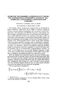
where (>1) is called price elasticity and γ (>0) is a scaling constant. The first three assumptions are the basic assumptions used in the classical EPQ model. The fourth assumption is based on the fact that to reduce the costs of production set-up and scrap and rework on shoddy protects substantial investment in improving the flexibility and reliability of the production process is necessary. The fifth assumption is mainly based on the unit variable production is demand dependent. When the demand of an item increases then the production/purchasing cost spread all over the items and hence the unit purchasing cost reduces and varies inversely with demand. The process reliability level r means of all the items produced in a production run only r % are acceptable quality that can be used to meet demand. The situation of the inventory model is illustrated in figure below:

Figure.1 Schematic of the situation of the economic production quantity model

2.3. Crisp Model If q(t) is the inventory level at time t over the time period (0, T), then

dq(t )  D for 0  t  T dt

(1.3)

with initial and boundary conditions q(0) = rq, q(T) = 0. The solution of this differential equation is obtained as q(t) = rq – Dt

(1.4)

and T = (rq) / D

(1.5)

Now, the inventory-carrying cost is given by JIC email for subscription: [email protected]

G.S. Mahapatra, et al: FUZZY PARAMETRIC GEOMETRIC PROGRAMMING WITH APPLICATION IN FUZZY

226

EPQ MODEL UNDER FLEXIBILITY AND RELIABILITY CONSIDERATION

hr 2 q 2  h  q(t )dt  h  (rq  Dt )dt  0 0 2D T

T

(1.6)

It is evident that the length of the production cycle is the sum of set-up, production, inventory carrying and interest and depreciation costs, that is total cost per cycle is S + pq + hq2 r2 / 2D + f(S, r)

(1.7)

Our objective is to minimize the total cost per unit time under limited budgetary cost. So TC (D, S, q, r) = (total cost per cycle) / (qr / D)

(1.8)

After substituting (1.1), (1.2) and (1.7) in (1.8) which becomes

TC ( D, S , q, r )  DSq 1r 1   D1  r 1 

Hqr  aDS  b q 1r  c 1 2

(1.9)

It is natural to expect the cost a product to be more if it is more sophisticated and reliable (except possible in the event of some major technological breakthrough). So, one can consider the budgetary function as an increasing function of reliability. Let the production cost per unit is Pr x and the total budgetary cost of the process is less or equal to B. Here we have considered budgetary cost as a constraint function as follows:

Pr x q  B

x   0,1

(1.10)

Hence the inventory model can be written as follows

Minimize TC ( D, S , q, r )  DSq 1r 1   D1  r 1  subject to

x

Hqr c 1  aDS  b q 1r   2

(1.11)

x   0,1

Pr q  B D, S, q, r >0

The above problem (1.11) can be treated as a Posynomial Geometric Programming problem with zero Degree of Difficulty.

2.4. Fuzzy Model If the coefficients of objective function and constraint goal of (1.11) are fuzzy [24] in nature then crisp model (1.11) transformed into a fuzzy model as follows

Minimize TC ( D , S , q , r )  DSq 1r 1   D 1  r 1  subject to

Pr x q  B 

x   0,1

 Hqr   b q 1r  c 1  aDS 2 (1.12)

D, S, q, r>0. where

 , h , a , P and B are fuzzy in nature.

3. Prerequisite Mathematics Definition 3.1 Fuzzy Set: A fuzzy set A in a universe of discourse X is defined as the following set

JIC email for contribution: [email protected]

Journal of Information and Computing Science, Vol. 7 (2012) No.3, pp 223-234

of pairs

A 

 x, 

A

 x   :x  X

. Here

 A : X   0,1

227

is a mapping called the membership function of

 x  the fuzzy set A and A is called the membership value or degree of membership of x X in the fuzzy  x   set A . The larger A is the stronger the grade of membership in A . Definition 3.2 Normal Fuzzy Set: A fuzzy set A of the universe of discourse X is called a normal fuzzy set implying that there exists at least one x X such that  A  x   1 . Otherwise the fuzzy set is subnormal.

Definition 3.3 -Level Set or -cut of a Fuzzy Set: The -level set (or interval of confidence at level  or -cut) of the fuzzy set A of X is a crisp set A that contains all the elements of X that have membership values in A greater than or equal to  i.e. A   x :  A  x    , x  X ,   [0,1]

Definition 3.4 Fuzzy Number: A fuzzy number A is a fuzzy set of the real line  whose membership function

 A ( x) has the following characteristics with   a1  a2  a3  a4    L ( x) for a1  x  a2  for a2  x  a3  1  A ( x)    R ( x) for a3  x  a4  0 for otherwise where  L ( x) :[a1,a2][0,1] is continuous and strictly increasing; strictly decreasing.

 R ( x) :[a3, a4][0, 1] is continuous and

4. Mathematical analysis Consider a particular non-linear programming problem

Min g0 ( x) s.t. g i ( x)  1

(4.1)

(1  i  n)

x > 0. Its objective and constraint functions are of the form Ti

m



gi ( x )   cik  x j ikj (0  i  n) k 1

j 1

where xj > 0; and cik, ρikj are real numbers. The constraint in (4.1) needs softening and considering the problem of fuzzy objective and constraint with fuzzy coefficients, we transform (4.1) into a fuzzy geometric programming [25] as follows:  g ( x) Min (4.2) 0

subject to gi ( x )  1 

(1  i  n),

x > 0,

JIC email for subscription: [email protected]

228

G.S. Mahapatra, et al: FUZZY PARAMETRIC GEOMETRIC PROGRAMMING WITH APPLICATION IN FUZZY

EPQ MODEL UNDER FLEXIBILITY AND RELIABILITY CONSIDERATION T

where x   x1 , x2 ,..., xm  is a variable vector, Ti

m



gi ( x )   cik  x j ikj k 1

(0  i  n) are all posynomial of x in which coefficients cik are fuzzy

j 1

numbers. Here for fuzzy numbers cik   c1ik , c2 ik , c3ik  containing the coefficients cik  0  i  n;1  k  Ti  , with the membership function as follow

 c2 ik  t  c  c for c1ik  t  c2ik  2 ik 1ik  t  c2ik cik  t    for c2ik  t  c3ik  c3ik  c2ik  0 otherwise   Here α-cut of cik  0  i  n;1  k  Ti  is given by

(4.3)

cik    cikL   , cikR      c1ik    c2ik  c1ik  , c3ik    c3ik  c2ik  

(4.4)

Proposition 4.1 If the coefficients of the fuzzy geometric programming problem are taken as fuzzy numbers then the problem (4.2) reduces to T0

Min

m



 c0kL   x j 0 kj k 1

(4.5)

j 1

Ti

Subject to

m



 cikL   x j ikj  1, k 1

1  i  n 

j 1

x j  0. If the coefficients are taken as fuzzy numbers then the fuzzy geometric programming problem (4.2) will take the form: T0 i

m

  Min  c0 k  x j 0 kj k 1

j 1

Ti

Subject to

m



cik  x j ikj  1, 1  i  n    k 1 j 1 x j  0.

Using α-cut of the fuzzy numbers coefficients, the above problem is reduces to T0

Min

m



 c0kL   , c0 kR    x j 0 kj k 1 Ti

Subject to

(4.6)

j 1 m

 c   , c    x ikL

ikR

k 1

j 1

ikj j

 1, 1  i  n  

x j  0. Which is equivalent to T0

Min

k 1

JIC email for contribution: [email protected]

m



 c0kL   x j 0 kj j 1

(4.7)

Journal of Information and Computing Science, Vol. 7 (2012) No.3, pp 223-234

Ti

Subject to

m

229



 cikL   x j ikj  1, k 1

1  i  n 

j 1

x j  0.

4.1. Solution procedure of fuzzy parametric geometric programming Solution of parametric problem (4.7) using fuzzy parametric geometric programming problem is discussed here. Problem (4.7) is a constrained posynomial GP problem. The number of terms in each posynomial constraint function varies and it is denoted by Tr for each r=0,1,2,…,l. Let T=T0+T1+T2+…+Tl be the total number of terms in the primal program. The Degree of Difficulty =T-(m+1). The dual problem of the primal problem (4.7) is as follows  rk

 rk

  crkL     Tr Maximize d ( )        rs   rk   s 1Tr 1 r  0 k 1   Tr

l

(4.8)

T0

subject to



0k

 1,

(Normality condition)

k 1 l

Tr

 

  0 , (j=1,2,...,m)

rkj rk

(Orthogonality conditions)

r  0 k 1

 rk  0 , (r=0,1,2,…,l; k=1,2,..,Tr).

(Positivity conditions) Case I. For T  m+1, the dual program presents a system of linear equations for the dual variables. A solution vector exists for the dual variables. Case II. For T0. Applying GP technique the dual programming of the problem (5.1) is 1

2

3

4

 1      (1)1     H0  (1 )H1     a0  (1 )a1   Max d( )     0      2 3 4  1       

5

  1    W0  (1)W1  

(5.2)

subject to

1   2   3   4  1 1  (1   ) 2   4  0 1  b 4  0 1   3   4   5  0 1   2   3  (c  1) 4  x 5  0

(5.3)

This is a system of five linear equations in five 5 unknowns. Solving we get the optimal values as follows

1* 

b( x  1)(   1) (1  b)(2 x   x  2)  c (   1)

(5.4)

 2* 

( x  1)(1  b) (1  b)(2 x   x  2)  c (   1)

(5.5)

 3* 

(1  b) (   1)( x  c)  2    (1  b)(2 x  x  2)  c (   1)

(5.6)

 4* 

( x  1)(   1) (1  b)(2 x  x  2)  c(   1)

(5.7)

 5* 

c(1   )  (1  b) ( x  1) ( x  1) (1  b)(2 x  x  2)  c (   1)

(5.8)

Putting these values in (5.1) we get the optimal solution of dual problem. The values of D, S, q, r is obtained by using the primal dual relation as follows From primal dual relation we get

DSq 1r 1  1*  d *   

 0  (1   ) 1  D1  r 1   2*  d *    H 0  (1   ) H1  qr   3*  d *    a0  (1   )a1  DS  b q 1r  c1   4*  d *   1 r x q   5* W  (1   ) W  0 1 The optimum solution of the model (1.12) through parametric approach is given by JIC email for contribution: [email protected]

Journal of Information and Computing Science, Vol. 7 (2012) No.3, pp 223-234

1

2

231

3

4

5

 1     (1)1   H0  (1)H1   a0  (1)a1    1 d ( )     0        2 3 4  1         W0  (1)W1  *

 c ( H 0  (1   ) H1 ) 5*  q   W0  (1   )W1    2 d * ( )   3*   * * 2  d ( )   3 r*  c ( H 0  (1   ) H1 ) 5* *

x

* 5

1

  1  2  (d * ( )) 2   3*   2* D  *  ( 0  (1   ) 1 )( H 0  (1   ) H1 )c 5  *

*

* 3

 2  d ( )    2  ( d * ( ))2   3*   2* S*   * ( H 0  (1   ) H1 )  ( 0  (1   ) 1 )( H 0  (1   ) H1 )c1 



1 1 

Note that optimal solution of GP technique in parametric approach is depends on α.

6. An illustrative example of the EPQ model A manufacturing company produces a machine. It is given that the inventory carrying cost of the machine is $10.5 per unit per year. The production cost of the machine varies inversely with the demand. From the past experience, the production cost of the machine is 15000D-3.6, where D is the demand rate. The total cost of interest and depreciation per production cycle is 1500S-1.6r, where S and r are set-up cost 0.6 per batch and production process reliability respectively. Let production cost per unit is 8r and total

budgetary cost (C) is $ 58. Determine the demand rate (D), set-up cost (S), production quantity (q), production process reliability (r), and optimum total average cost (TC) of the production system. Formulation of the said model is presented as follows:

Min TC(D, S, q, r)  DSq1r1 15000D13.6r 1  subject to

8 r 0.6 q  58

10.5qr 1.51 1500DS 1.6q1r  2 x  0,1

(6.1)

The optimum solution of the problem (6.1) by Non-Linear programming (NLP) and Geometric Programming (GP) using LINGO [26] are presented in Table 1. Method GP NLP

Table 1 Optimal solution of EPQ model (6.1) TC*($) D* S*($) q* r* 114.1258 14.56821 14.91823 9.679971 0.6053934 114.1618 14.65152 14.93629 9.799638 0.6051736

  14900  1    250 , 5.25   5  1    0.5 , When the coefficient are taken as fuzzy number i.e. 15000   1475  1    50 , 8  8  1    0.275 and 58  58  1    2,    0,1 the optimal solutions of the 1500

fuzzy model by fuzzy parametric geometric programming is presented in table 2.

JIC email for subscription: [email protected]

232

G.S. Mahapatra, et al: FUZZY PARAMETRIC GEOMETRIC PROGRAMMING WITH APPLICATION IN FUZZY

EPQ MODEL UNDER FLEXIBILITY AND RELIABILITY CONSIDERATION

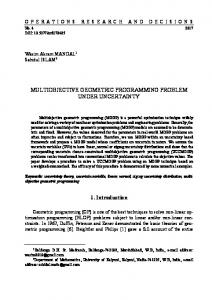
α 0.1 0.2 0.3 0.4 0.5 0.6 0.7 0.8 0.9 1.0

Table 2 Optimal solution of fuzzy EPQ model of (6.1) TC ($) D* S*($) q* 114.9443 15.54715 13.74584 11.07385 114.6381 15.40587 13.92585 10.87414 114.3301 15.26491 14.10965 10.67673 114.0201 15.12427 14.29737 10.48161 113.7083 14.98395 14.48912 10.28876 113.3945 14.84396 14.68502 10.09816 113.0788 14.70428 14.88520 9.909811 112.7610 14.56492 15.08978 9.723689 112.4412 14.42587 15.29892 9.539781 112.1193 14.28714 15.51275 9.358073 *

r* 0.5194229 0.5324381 0.5458799 0.5597660 0.5741147 0.5889454 0.6042784 0.6201351 0.6365380 0.6535106

The solution of objective function and decision variables for different value of α is shown by graphical presentation in figure 2.

Figure 2 Optimal objective value, decision variables D, S, q and r vs. α

7. Sensitivity analysis The change of optimal solutions of the problem for fuzzy model with small change of tolerance of constraint goal when α change is, given in Table 3. Table 3 shows that as B changes increasingly the total average cost of the given problem slightly decreases, which is expected. So it is clear from the sensitivity analysis that if the management traced on proceed reliability, the D and q will be less, so they should not the over 1000 demand. Another fact is that if production management decided on the fact they should try to fulfill the demand then the fact is on to be relation on the production process reliability and setup cost with changing of tolerance of constraint goal, decision variables are also changed. It is noted that the demand and order quantity are increasing with increasing tolerance of constraint goal but setup cost and process reliability are decreasing when tolerance increasing.

JIC email for contribution: [email protected]

Journal of Information and Computing Science, Vol. 7 (2012) No.3, pp 223-234

233

Table 3 Change of value of objective function and decision variables for change of α

α

0.1

0.3

0.5

0.7

0.9

Tolerance of B 0.25 0.5 0.75 0.25 0.5 0.75 0.25 0.5 0.75 0.25 0.5 0.75 0.25 0.5 0.75

TC*($)

D*

S*($)

Q*

r*

114.9443 114.0867 113.2600 114.3301 113.6595 113.0079 113.7083 113.2267 112.7551 113.0788 112.7883 112.5014 112.4412 112.3438 112.2469

15.54715 16.15895 16.77616 15.26491 15.73480 16.20798 14.98395 15.31532 15.64837 14.70428 14.90053 15.09737 14.42587 14.49043 14.55505

13.74584 13.02879 12.36821 14.10965 13.52818 12.98311 14.48912 14.05581 13.64229 14.88520 14.61377 14.34996 15.29892 15.20440 15.11079

11.07385 12.06080 13.10344 10.67673 11.41730 12.19061 10.28876 10.79881 11.32508 9.909811 10.20473 10.50531 9.539781 9.634461 9.729751

0.5194229 0.4733597 0.4325368 0.5458799 0.5074780 0.4725617 0.5741147 0.5446813 0.5172066 0.6042784 0.5853072 0.5671140 0.6365380 0.6297368 0.6230312

8. Conclusion In this paper, an economic production quantity model with investment costs for set-up reduction and quality improvement is formulated. The model has involved one budgetary constraint. The problem is solved by Fuzzy parametric GP method. The Fuzzy parametric GP method provides an alternative approach to this problem. The method, as illustrated, is efficient and reliable. Here decision maker may obtain the optimal results according to his expectation. The method presented is quite general and can be applied to the model in other areas of operation research and other field of optimization involvement.

9. References [1] R.J. Duffin, E.L. Peterson, C. Zener, Geometric Programming–theory and application, John wiley, New York, 1967. [2] E.L. Peterson, Geometric programming, Siam Review. 18 (1974) 37-46. [3] M.J. Rijckaert, Survey of programs in geometric programming, C.C.E.R.O. 16 (1974) 369-382. [4] T.R. Jefferson and C. H. Scott, Avenues of geometric programming, New Zealand Operational Research. 6 (1978) 109-136. [5] T.C.E. Chang, An economic production quantity model with flexibility and reliability considerations, European Journal of Operational Research 39 (1989) 174-179. [6] T.C.E. Chang, An economic production quantity model with demand-dependent unit cost, European Journal of Operational Research 40 (1989) 252-156. [7] T.C.E. Cheng, An economic order quantity model with demand-dependent unit production cost and imperfect production processes. IIE Transactions 23, (1991a), 23–28. [8] iH. Jung, C.M. Klein, Optimal inventory policies for an economic order quantity model with decreasing cost functions, European Journal of Operational Research 165, (2005) 108–126.

JIC email for subscription: [email protected]

234

G.S. Mahapatra, et al: FUZZY PARAMETRIC GEOMETRIC PROGRAMMING WITH APPLICATION IN FUZZY

EPQ MODEL UNDER FLEXIBILITY AND RELIABILITY CONSIDERATION [9] G.A. Kochenberger, Inventory models: Optimization by geometric programming. Decision Sciences 2, (1971) 193–205 [10] W.J. Lee, Determining order quantity and selling price by geometric programming: Optimal solution, bounds, and sensitivity. Decision Science 24, (1993) 76–87. [11] B.M. Worrall, M.A. Hall, The analysis of an inventory control model using posynomial geometric programming. International Journal of Production Research 20, (1982) 657–667. [12] [A.J. Clark, An informal survey of multi-echelon inventory theory. Naval Research Logistics Quarterly 19, (1972) 621–650. [13] G. Urgeletti, Inventory control: models and problems, European Journal of Operational Research 14 (1983) 1-12. [14] A.F. Veinott, The status of mathematical inventory theory. Management Science 12, (1966) 745–777. [15] A.C. Hax, D. Canada, Production and Inventory Management. Prentice-Hall, New Jersey 1984. [16] B.P. Van, C. Putten, OR contributions to flexibility improvement in production/inventory systems. European Journal of Operational Research 31, (1987) 52–60. [17] E.L. Porteus, Investing in reduced set-ups in the EOQ model. Management Science 31, (1985) 998–1010. [18] E.L. Porteus, Optimal lot sizing, process quality improvement and set-up cost reduction. Operations Research 34, (1986) 137–144. [19] M.J. Rosenblatt, H.L. Lee, Economic production cycles with imperfect production processes. IIE Transactions 18, (1986) 48–55 [20] W.I. Zangwill, From EOQ to ZI. Management Science 33, (1987) 1209–1223. [21] P.K. Tripathy, W.M. Wee, P.R. Majhi, An EOQ model with process reliability considerations. Journal of the Operational Research Society 54, (2003) 549–554. [22] S Islam, T.K. Roy, A fuzzy EPQ model with flexibility and reliability consideration and demand dependent unit production cost a space constraint : A fuzzy geometric programming approach, Applied Mathematics and computation 176 (2006) 531-544 . [23] K.N.F. Leung, A generalized geometric-programming solution to ‘An economic production quantity model with flexibility and reliability considerations’ European Journal of Operational Research 176 (2007) 240–251. [24] L.A. Zadeh, Fuzzy sets, Information and Control 8 (1965) 338-353. [25] B.Y. Cao, Fuzzy geometric programming. Series: Applied Optimization Vol.76: Kluwer Academic Publishers, Dordrecht, 2002. [26] LINGO: the modeling language and optimizer (1999). Lindo system Inc., Chicago,IL 60622, USA.

JIC email for contribution: [email protected]